ACU-T: 4001 Water Filling in a Tank
This tutorial provides the instructions for setting up, solving and viewing results for a transient simulation of a two-phase flow in a square tank using the level set model. In this simulation, AcuSolve is used to compute the time-varying water-level interface due to presence of water through the inlet and the outlet of the tank. This tutorial is designed to introduce you to a number of modeling concept necessary to perform two-phase simulations.
- Two-phase flow solution
- Transient simulation
- Use of a script for the water volume fraction initialization
- Post-processing with AcuFieldView
Prerequisites
You should have already run through the introductory tutorial, ACU-T: 2000 Turbulent Flow in a Mixing Elbow. It is assumed that you have some familiarity with AcuConsole, AcuSolve, and AcuFieldView. You will also need access to a licensed version of AcuSolve.
Prior to running through this tutorial, copy AcuConsole_tutorial_inputs.zip from <Altair_installation_directory>\hwcfdsolvers\acusolve\win64\model_files\tutorials\AcuSolve to a local directory. Extract tank2D.x_t from AcuConsole_tutorial_inputs.zip.
Analyze the Problem
An important step in any CFD simulation is to examine the engineering problem at hand and determine the important parameters that need to be provided to AcuSolve. Parameters can be based on geometrical elements (such as inlets, outlets, or walls) and on flow conditions (such as fluid properties, velocity).
In general, multiphase flows are mainly observed in real life environment, consisting of two or more fluids (gas, liquid, or solid). They have possible combinations of gas-liquid (dissolved gas), liquid-liquid (oil in water), liquid-solid (immersed particles), as well as gas-liquid-solid. The first two are examples of two-phase immiscible flows. The two-phase immiscible flows can be solved by tracking the interface between the two-phases. This tutorial will guide you through how to set up the two-phase flow problem using the level set method.

Figure 1. Schematic of the Problem
Define the Simulation Parameters
Start AcuConsole and Create the Simulation Database
In this tutorial, you will begin by creating a database, populating the geometry-independent settings, loading the geometry, creating volume and surface groups, setting group parameters, adding geometry components to groups, and assigning mesh controls and boundary conditions to the groups. Next you will generate a mesh and run AcuSolve to solve for the number of time steps specified. Finally, you will visualize some characteristics of the results using AcuFieldView.
In the next steps you will start AcuConsole, and create the database for storage of the simulation settings.
Set General Simulation Parameters
In next steps you will set parameters that apply globally to the simulation. To make this simple, the basic settings applicable for any simulation can be filtered using the BAS filter in the Data Tree Manager. This filter enables display of only a small subset of the available items in the Data Tree and makes navigation of the entries easier.
-
Click BAS in the Data Tree Manager to switch to basic view in the Data Tree.
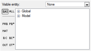
Figure 2. -
Double-click the Global
Data Tree item to expand it.
Tip: You can also expand a tree item by clicking
 next to the item name.
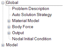
Figure 3. -
Ensure that Multiphase equation is set to Level
Set.
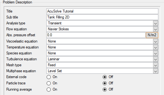
Figure 4.
Set Solution Strategy Parameters
-
Change Fluid 2 to Air.
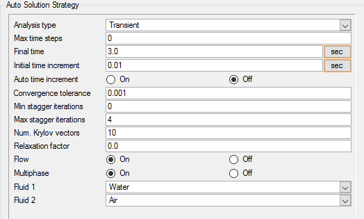
Figure 5.
Set Material Model Parameters
-
Double-click Material Model
in the Data Tree to expand it.
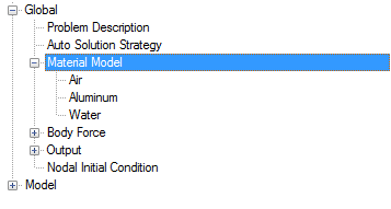
Figure 6.
The remaining thermal and other material properties are not critical to this simulation. However, you may browse through the tabs to check the complete material specification
-
Save the database to create a backup
of your settings. This can be achieved with any of the following
methods.
- Click the File menu, then click Save.
- Click
 on
the toolbar.
on
the toolbar. - Click Ctrl+S.
Note: Changes made in AcuConsole are saved into the database file (.acs) as they are made. A save operation copies the database to a backup file, which can be used to reload the database from that saved state in the event that you do not want to commit future changes.
Set the Multiphase Parameters
When Multiphase is activated in the Problem Description, by selecting a Multiphase equation, AcuConsole automatically generates the necessary set of parameters required to complete the multiphase model definition. These include defining the fields in the model, and also specifying the interaction models between the fields.
In this section you will define the multiphase parameters for the simulation.
-
Define the fields:
- Click on ALL in the Data Tree Manager to display all available simulation settings.
- Expand the Data Tree item.
- Under Multiphase Parameters, expand the Fields item.
- Double-click Air.
- Set Modify advanced settings to On and check that the Material model is set to Air.
- Double-click Water.
- Set Modify advanced settings to On and check that the Material model is set to Water.
-
Define the Field Interaction Model:
- Under Multiphase Parameters, expand the Field Interaction Model item.
- Right-click on Air-Water and click Delete.
- Double-click Water-Air to open the detail panel.
- Set Modify advanced settings to On.
- Click Open Refs next to Fields 1.
- Check that the entry in the Reference Editor is Water.
- Click Open Refs next to Fields 2.
- Check that the entry in the Reference Editor is Air.
- Set the Surface tension model to None.
- Set the Thickness type to Auto.
-
Define the Multiphase Model:
- Under Multiphase Parameters, expand the Multiphase Model item.
- Right-click on Air-Water and select Delete.
- Double-click Water-Air to open the detail panel.
- Set Modify advanced settings to On.
- Click Open Refs next to Field interaction models.
- Check that the entry in the Reference Editor is Water-Air.
Import the Geometry and Define the Model
Import the Geometry
-
Select tank2D.x_t and click
Open to open the Import Geometry
dialog.
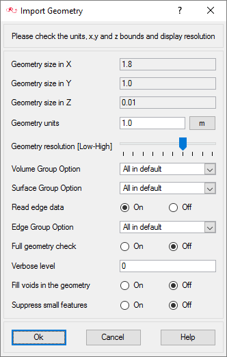
Figure 7.For this tutorial, the default values for the Import Geometry dialog are used to load the geometry. If you have previously used AcuConsole, be sure that any settings that you might have altered are manually changed to match the default values shown in the figure. With the default settings, volumes from the CAD model are added to a default volume group. Surfaces from the CAD model are added to a default surface group. You will work with groups later in this tutorial to create new groups, set flow parameters, add geometric components, and set meshing parameters.
-
Click Ok to complete
the geometry import.

Figure 8.
Set the Body Force
The body force commands add volumetric source terms to the governing conservation equations. In this tutorial, gravitational body force will be applied to the fluid fields. Gravity will be defined as equal to standard gravity (g = 9.81 m/s2) along the negative Y-axis, which is the downward direction in the model.
Define Nodal Outputs
The nodal output command specifies the nodal output parameters, for example, output frequency and number of saved states.
-
Make sure that the Number of saved states is set to
0.
Setting this option to zero will instruct the solver to save all of the solution state files.
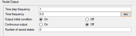
Figure 9.
Set the Initial Conditions
Apply Volume Parameters
Volume groups are containers used for storing information about a volume region. This information includes solution and meshing parameters applied to the volume and the geometric regions that these settings are applied to.
When the geometry was imported into AcuConsole, all volumes were placed into the "default" volume container.
Since the model for this tutorial has only a single volume, it will be the only volume in the default volume group when the geometry is imported. Even when there is a single volume in the model, it is advisable to rename the volume for ease of identification in future. In the next steps you will rename the default volume group container, and set the material and other properties for it.
-
Expand Volumes. Toggle the display of the default
volume container by clicking
 and
and  next to the volume name.
Note: You may not see any change when toggling the display if Surfaces are being displayed, as surfaces and volumes may overlap.
next to the volume name.
Note: You may not see any change when toggling the display if Surfaces are being displayed, as surfaces and volumes may overlap. -
Set up the Fluid volume element set.
- Expand Fluid in the Data Tree.
- Double-click Element Set under Fluid to open it in the detail panel.
- For Medium, select Multiphase.
- For Multiphase model, select Water-Air.
- For Body force, select Gravity.
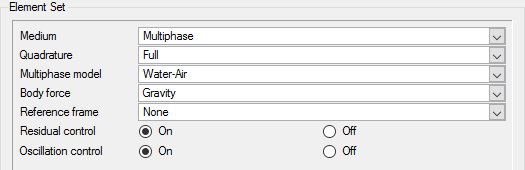
Figure 10.
Create Surface Groups and Apply Surface Attributes
Surface groups are containers used for storing information about a surface, including solution and meshing parameters, and the corresponding surface in the geometry that the parameters will apply to.
In the next steps you will define surface groups, assign the appropriate settings for the different characteristics of the problem, and add surfaces to the group containers.
In the process of setting up a simulation, you need to move into different panels for setting up the boundary conditions, mesh parameters, and so on, which can sometimes be cumbersome (especially for models with too many surfaces). To make it easier, less error prone, and for saving time two new dialogs are provided in AcuConsole which you can use to verify and provide the information for all surface or volume entities at once. They are the Volume Manager and Surface Manager. In this section some features of the Surface Manager are exploited.
-
Rename Surface Names (column 1) for Surface 1 to Surface 5, and set the Simple
BC Active and Simple BC Type columns as per the table shown below.
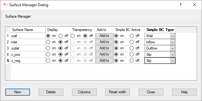
Figure 11. -
Assign the surfaces to the z_pos and z_neg surface groups.
-
Similarly assign the surface with the minimum z-coordinate to the z_neg
surface group.
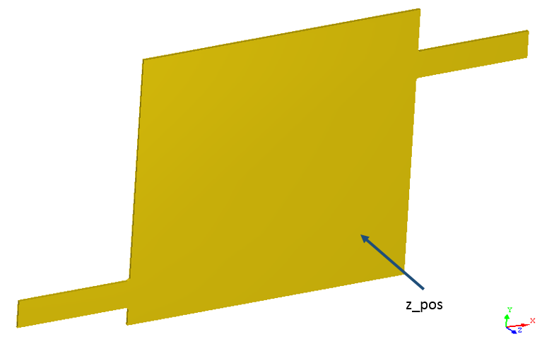
Figure 12.
-
Similarly assign the surface with the minimum z-coordinate to the z_neg
surface group.
-
Assign the surface with the minimum x-coordinate to
outlet surface group.
Use the following figure as the reference for selecting the required surfaces.
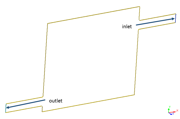
Figure 13.When the geometry was loaded into AcuConsole, all geometry surfaces were placed in the default surface group container. This default surface group was renamed to sides. In the previous steps, you assigned some surfaces to various other surface groups that you created. At this point, all that is left in the sides surface group are the surfaces which make up the sides of the reservoir.
Inlet
As mentioned earlier, the inlet in this problem is a water inlet with inlet velocity set as 1.5 m/s.
-
Set the Incoming fluid field to Water from the drop down
selector menu.
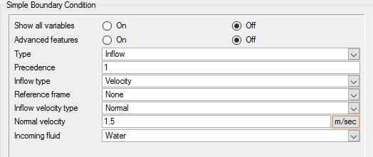
Figure 14.
Outlet
-
Click Open Array next to Hydrostatic pressure origin to
check that the origin location is at (0, 0, 0)
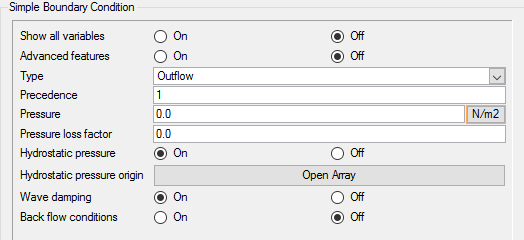
Figure 15.
Wall
-
Check that the Type is set to Wall.
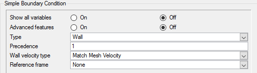
Figure 16.
z_pos and z_neg
- In the Data Tree, under Surfaces, expand the z_pos surface.
- Double-click Simple Boundary Condition to open the detail panel.
- Check that the Type is set to Slip.
- Similarly, check that the Simple Boundary Condition type for z_neg is also set to Slip.
Assign Mesh Controls
Set Global Meshing Attributes
Now that the flow characteristics have been set for the whole problem, a sufficiently refined mesh has to be generated.
Global mesh attributes are the meshing parameters applied to the model as a whole without reference to a specific geometric volume, surface, edge, or point. Local mesh attributes are used to create mesh generation controls for specific geometry components of the model.
In the next steps you will set the global mesh attributes.
-
Set Absolute mesh size to 0.12.
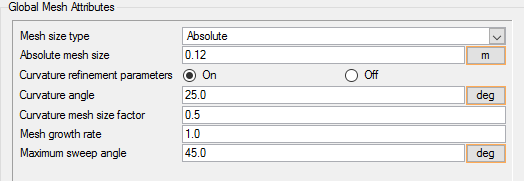
Figure 17.
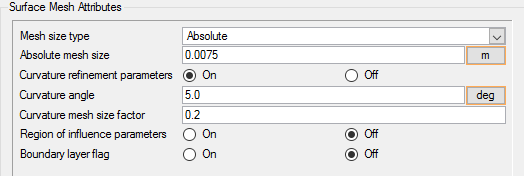
Set Surface Mesh Parameters
Surface mesh attributes are applied to a specific surface in the model. It is a type of local meshing parameter used to create targeted mesh controls for one or more specific surfaces.
Setting local mesh attributes, such as surface mesh attributes, is not mandatory. When a local mesh attribute is not found for a component, the global attributes are used as the mesh generation control for that component. If a local mesh attribute is present, it will take precedence over the global setting.
In the next steps you will set the surface meshing attributes.
-
Set the Curvature mesh size factor to 0.2.
This setting is used to determine the minimum value of the mesh edge length used to resolve curved features. This minimum value is computed by multiplying the Absolute or Relative mesh size with the Curvature mesh size factor.
Set Zone Meshing Parameters
In the last section, it was mentioned that surface mesh attributes are local mesh attributes that are applied to a specific surface. Similarly, there is a provision for edge mesh attributes that are local to a specific edge in the model. However, at times it is desired to specify a mesh attribute local to a region independent of the CAD entities in the model. This can be achieved using Zone Mesh Attributes. It is possible to specify a zone in the shape of a box, cylinder or a sphere for example, with local mesh control attributes to be used within that zone. Wherever this zone overlaps the CAD model, the zonal mesh attributes will be used instead of the global mesh attributes.
In the following steps, you will define a mesh refinement zone, and set up the zonal mesh attributes for it to be used in the model. A box-shaped refinement zone will be used in the region where a water-air interface is expected.
-
Enter the values in the Array Editor
as shown below and click OK.
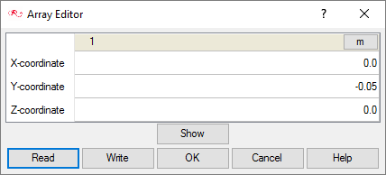
Figure 18. -
Set the Mesh size to 0.015 m
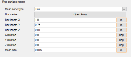
Figure 19.
Figure 20.
Define Mesh Extrusion
The present simulation is equivalent to a representation of a 2D cross section of the model. In AcuSolve 2D models are simulated by having just one element across the faces of the cross section. Thus when these faces are set up with a similar boundary condition, it coerces the corresponding nodes across the faces to have same results. In this problem, these faces are the negative and positive z-surfaces. This kind of mesh is achieved in AcuSolve with mesh extrusion process. In the following steps you will define the process of extrusion of the mesh between these surfaces.
-
Click OK to accept these settings.
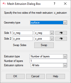
Figure 21.
Generate the Mesh
In the next steps you will generate the mesh that will be used when computing a solution for the problem.
-
Click
 on the toolbar to open the Launch
AcuMeshSim dialog.
on the toolbar to open the Launch
AcuMeshSim dialog.
-
Leave the default settings and select OK.
When AcuFieldView is started directly from AcuConsole, the model will be displayed in an isometric view with a Boundary Surface dialog open. The initial view is shown in perspective, with an outline around the model. You will manipulate the view in the next steps, and in later steps will view different flow characteristics using the Boundary Surface dialog.
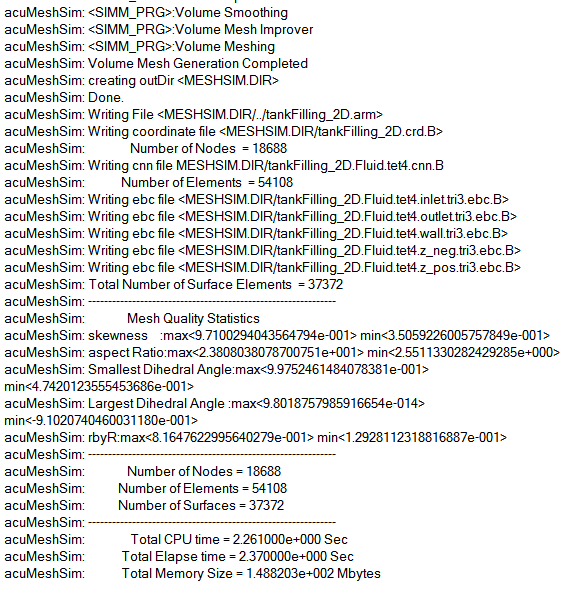
Figure 22.Note: The actual number of nodes and elements, and memory usage may vary slightly from machine to machine.
Compute the Solution and Review the Results
Run AcuSolve
In the next steps, you will launch AcuSolve to compute the solution for this case.
-
Click
 on the toolbar to open the
Launch AcuSolve dialog.
on the toolbar to open the
Launch AcuSolve dialog.
For this case, the default settings will be used. AcuSolve will run using four processors (if available, higher number of processors may be specified) and AcuConsole will generate AcuSolve input files and will launch AcuSolve. AcuSolvewill calculate the steady state solution for this problem.
Post-Process with AcuFieldView
- How to find the data readers in the File menu and open up the desired reader panel for data input.
- How to find the visualization panels either from the Side toolbar or the Visualization panel menu to create and modify surfaces in AcuFieldView
- How to move the data around the graphics window using mouse actions to translate, rotate and zoom in to the data.
-
Click
 on the
AcuConsole toolbar to open the
Launch AcuFieldView dialog.
You will see that the pressure contours have already been displayed on all the boundary surfaces with mesh.
on the
AcuConsole toolbar to open the
Launch AcuFieldView dialog.
You will see that the pressure contours have already been displayed on all the boundary surfaces with mesh. -
Click OK to start AcuConsole.
You will see that the pressure contours have already been displayed on all the boundary surfaces with mesh.
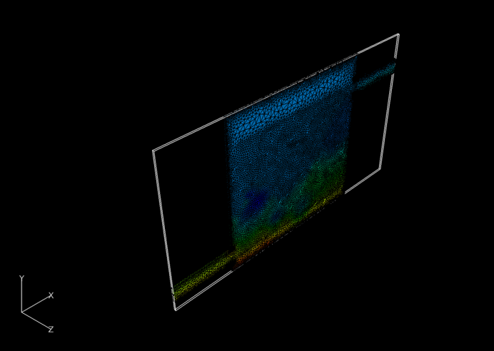
Figure 23.
Set Up AcuFieldView
-
Click Viewer Options.
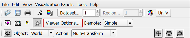
Figure 24. -
On the toolbar, click the Colormap icon
 .
.
-
Click the Toggle Outline icon
 on the toolbar to turn off the outline display.
Your display should look similar to figure 1.
on the toolbar to turn off the outline display.
Your display should look similar to figure 1.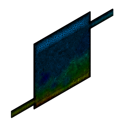
Figure 25.
Coordinate the Surface Showing Water-Air Interface on the Mid Coordinate Surface
-
Click
 to open
the Coordinate Surface dialog.
to open
the Coordinate Surface dialog.
-
From the Defined Views list, select +Z as the viewing
direction.
Your view should be similar to Figure 26.
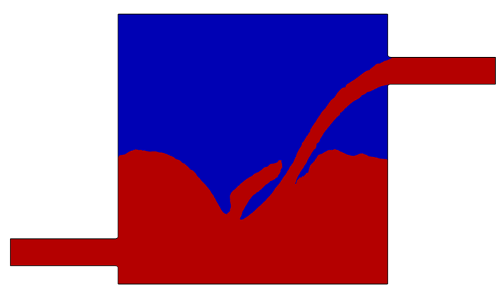
Figure 26.
Visualize the Animation of the Water Flow
If the Sweep Control in this dialog says Sweep instead of Build, the Flipbook Build Mode is not active. In Sweep mode, you will be able to create and visualize the animation but you will not be able to save it. To be able to save the animation, enable the Flipbook Build Mode.
-
Click Apply.
The displayed state now corresponds to the initial state of the domain.
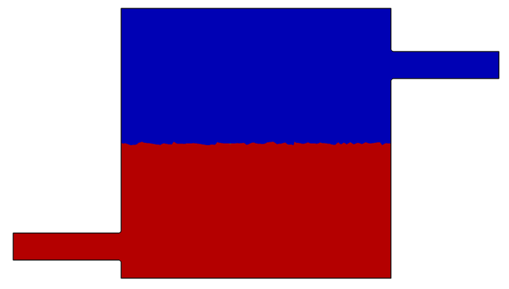
Figure 27. -
Click Play
 to play the animation.
-
To save the animation, click Pause
 , and then click
Save.
, and then click
Save.
Summary
In this AcuSolve tutorial, you successfully set up and solved a multiphase flow problem. The problem simulated a square shaped water tank in which water was being injected through an inlet. The tank also had an open outlet. As the water filled in through the inlet, the air-water interface in the tank was visualized. You started the tutorial by creating a database in AcuConsole, importing and meshing the geometry, and setting up the simulation parameters. Air and water were modelled as different fields occupying a single volume. Once the case was setup, the solution was generated with AcuSolve. Results were post-processed in AcuFieldView where you generated an animation of the water flow. New features that were introduced in this tutorial include: setting up a multiphase flow simulation in AcuSolve with two fluids.