ACU-T: 3311 Multiphase Nucleate Boiling Using the Algebraic Eulerian Model
This tutorial provides instructions for modeling a two-phase nucleate boiling in a pipe using the Algebraic Eulerian model. Prior to starting this tutorial, you should have already run through the introductory HyperWorks tutorial, ACU-T: 1000 HyperWorks UI Introduction, and have a basic understanding of HyperWorks CFD and AcuSolve. To run this simulation, you will need access to a licensed version of HyperWorks CFD and AcuSolve.
Prior to running through this tutorial, copy HyperWorksCFD_tutorial_inputs.zip from <Altair_installation_directory>\hwcfdsolvers\acusolve\win64\model_files\tutorials\AcuSolve to a local directory. Extract ACU-T3311_TwoPhaseNB.hm from HyperWorksCFD_tutorial_inputs.zip.
Problem Description
The problem to be addressed in this tutorial is shown schematically in Figure 1. It consists of a channel with a heated wall at the bottom. The temperature of the wall is selected to onset the nucleate boiling at the heated wall.
Water at 2 bar pressure and 95 ℃ temperature enters the inlet at an average velocity of 0.39 m/sec and passes through the heated wall which is maintained at 130 ℃.
The pre-heated air enters the inlets and heat is transferred to the fluid from the walls. The heat causes sub-cooled boiling to occur in the region close to the wall and leads to formation of bubbles at nucleation sites.
The heat transfer in this regime is basically dominated by two effects, the macro convection due to the motion of the bulk liquid and the latent heat transport associated with the evaporation of the liquid micro-layer between the bubble and the heated wall.

Figure 1. Schematic of Channel
Start HyperWorks CFD and Open the HyperMesh Database
-
From the Home tools, Files tool group, click the Open Model tool.

Figure 2.The Open File dialog opens.
Validate the Geometry
The Validate tool scans through the entire model, performs checks on the surfaces and solids, and flags any defects in the geometry, such as free edges, closed shells, intersections, duplicates, and slivers.
Figure 3.
Set Up Flow
Verify and Create Materials
-
From the Flow ribbon, click the Material Library tool.

Figure 4.The Material Library dialog opens. -
Verify that the material Water_NB has the properties shown below.
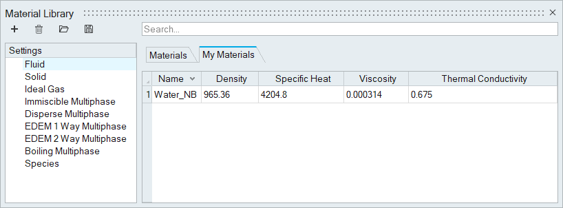
Figure 5. -
Click
 to create a new material.
-
Name the material Boiling_NB and verify the following
properties in the microdialog.
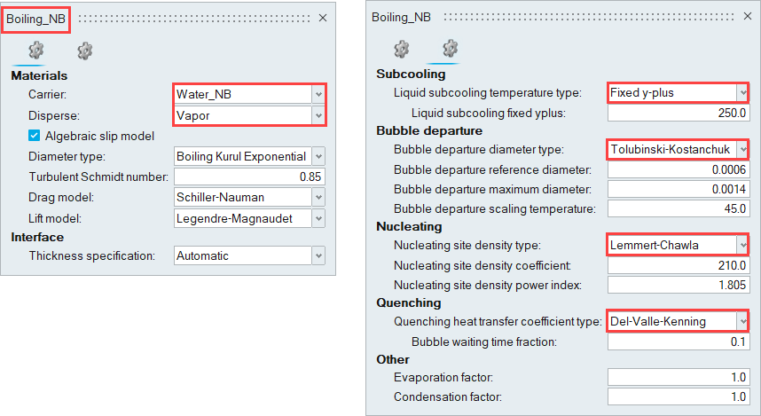
Figure 6.
Set the General Simulation Parameters
-
From the Flow ribbon, click the Physics tool.

Figure 7.The Setup dialog opens. -
Under the Physics models setting:
- Activate the Multiphase flow radio button.
- Set the Multifluid type to Boiling and the Boiling material to Boiling_NB.
- Ensure that the Time step size is 0.01.
- Select Spalart-Allmaras as the Turbulence model.
- Set the Gravity value to -9.81 in the z direction.
-
Set the Pressure scale to Gauge then click
 besides the drop-down and set the Absolute
pressure offset to 200000.
besides the drop-down and set the Absolute
pressure offset to 200000.
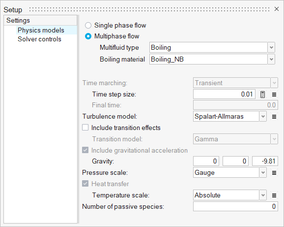
Figure 8. -
Click the Solver controls setting and verify that:
- Minimum stagger iteration is set to 2.
- Maximum stagger iteration is set to 4.
- Transient maximum step is set to 40.
- The Flow, Temperature, Multifluid, and Turbulence checkboxes are activated.
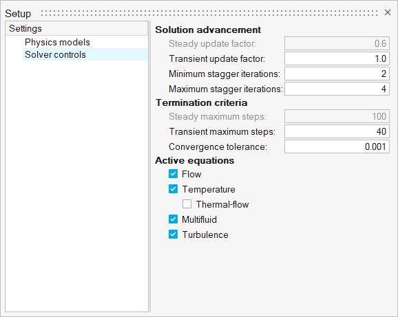
Figure 9.
Assign Material Properties
-
From the Flow ribbon, click the Material tool.

Figure 10. -
Select Boiling_NB from the Material drop-down
menu.
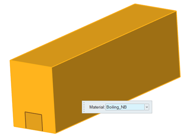
Figure 11. -
On the guide bar, click
 to execute
the command and exit the tool.
to execute
the command and exit the tool.
Define Flow Boundary Conditions
-
From the Flow ribbon, Profiled
tool group, click the Profiled Inlet tool.

Figure 12. -
In the microdialog, enter 0.39
as the Average velocity.
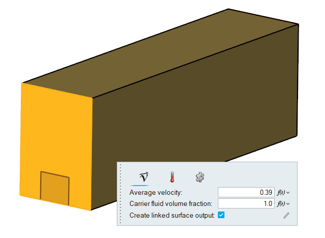
Figure 13. -
Click the Temperature tab in the microdialog and enter
368.15.
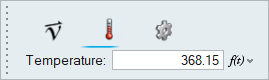
Figure 14. -
On the guide bar, click
to execute
the command and exit the tool.
-
Click the Outlet tool.

Figure 15. -
Select the face highlighted in the figure below then click
 on the
guide bar.
on the
guide bar.
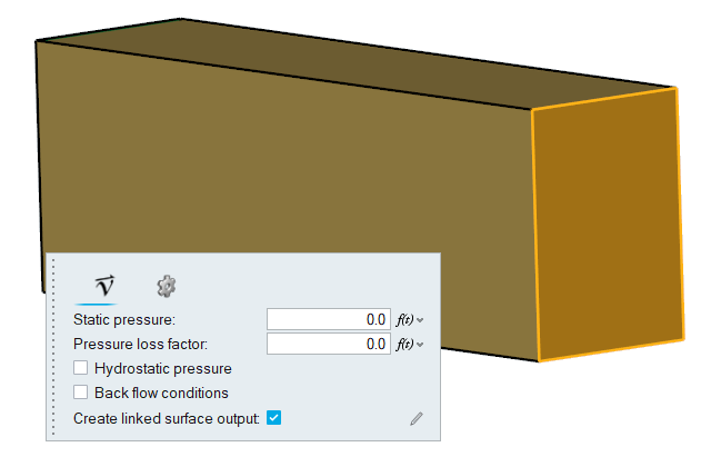
Figure 16. -
Click the No Slip tool.

Figure 17. -
Select the face highlighted in the figure below to create the Heated_wall
face.
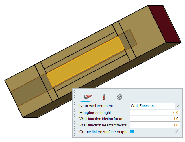
Figure 18. -
Click the Temperature tab in the microdialog, set the
Thermal Boundary condition to Temperature, and set the
Temperature value to 403.15.
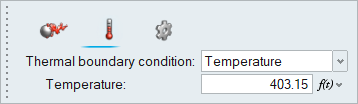
Figure 19. -
On the guide bar, click
 to execute the command and remain in the
tool.
to execute the command and remain in the
tool.
-
In the Boundaries legend, right-click on Wall, select
Rename, and enter
Heated_wall.
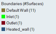
Figure 20. -
Select the 8 highlighted surfaces shown in the figure below to create the
Bottom_wall faces then click
 on the guide bar.
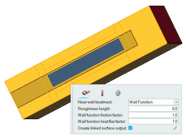
Figure 21. -
From the Solution ribbon, click the Field tool.

Figure 22.The Field Output dialog opens. -
Set the Time step interval to 10.
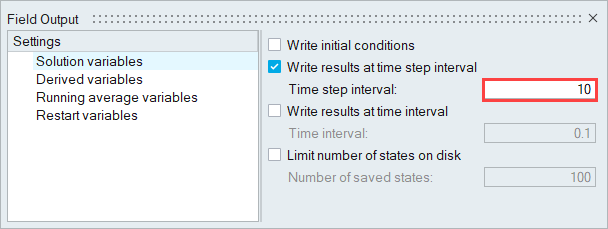
Figure 23.
Generate the Mesh
-
From the Mesh ribbon, click the Batch tool.

Figure 24. -
In the Meshing Operations dialog, set the Average Element
size to 0.004 (if not set already).
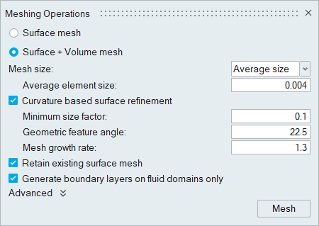
Figure 25.
Run AcuSolve
-
From the Solution ribbon, click the Run tool.

Figure 26.The Launch AcuSolve dialog opens. -
Expand Default initial conditions and enter the values
as shown below to define the initial conditions.
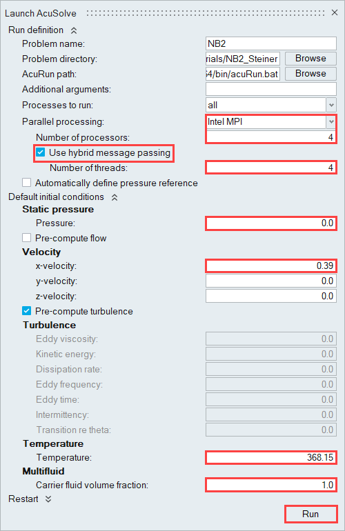
Figure 27.
Post-Process the Results with HW-CFD Post
-
Select the AcuSolve log file in your problem
directory to load the results for post-processing.
The solid and all the surfaces are loaded in the Post Browser.
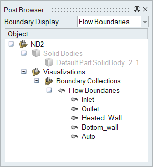
Figure 28. -
From the Post ribbon, click the Boundary Groups tool.

Figure 29. -
Activate the Legend radio button then click
 and set the legend properties as
shown below.
and set the legend properties as
shown below.
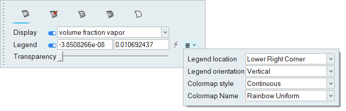
Figure 30. -
Click on the guide bar.
The volume fraction of vapor contours are displayed on the model.
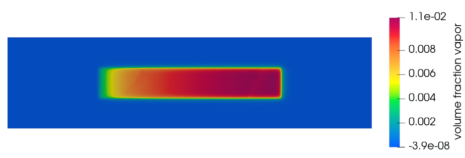
Figure 31.
Summary
In this tutorial, you successfully learned how to set up and solve a simulation involving a two-phase nucleate boiling using HyperWorks CFD. You started by opening the HyperMesh input file with the geometry and then defined the simulation parameters and flow boundary conditions. Once the solution was computed, you used HW-CFD post to create the contours of volume fraction of vapor.