ACU-T: 3300 Modeling of a Heat Exchanger Component
Prerequisites
This tutorial provides instructions for running a steady-state simulation of a flow inside a pipe with an interior heat exchanger placed at the middle of the pipe. Prior to starting this tutorial, you should have already run through the introductory HyperWorks tutorial, ACU-T: 1000 HyperWorks UI Introduction, and have a basic understanding of HyperMesh and AcuSolve. To run this simulation, you will need access to a licensed version of HyperMesh and AcuSolve.
Prior to running through this tutorial, copy HyperMesh_tutorial_inputs.zip from <Altair_installation_directory>\hwcfdsolvers\acusolve\win64\model_files\tutorials\AcuSolve to a local directory. Extract ACU-T3300_HeatExchanger.hm from HyperMesh_tutorial_inputs.zip.
Since the HyperMesh database (.hm file) contains meshed geometry, this tutorial does not include steps related to geometry import and mesh generation.
Problem Description
The problem to be addressed in this tutorial is shown schematically in the figure below. It consists of a cylindrical pipe channel with an interior heat exchanger component volume with thickness ‘t’ and radius ‘r’. The heat exchanger component parameters are assigned to the HEX_Inlet surface component. Basically, the heat exchanger model is applied to a surface and the temperature rises across that surface to model the effect of the heat exchanger. Air enters the pipe at a velocity of 0.1 m/sec and flows through the heat exchanger volume and then exits through the outlet.
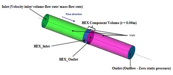
Figure 1.
Open the HyperMesh Model Database
-
Click the Open Model icon
 located on the standard toolbar.
The Open Model dialog opens.
located on the standard toolbar.
The Open Model dialog opens.
Set the General Simulation Parameters
In this step, you will set the simulation parameters that apply globally to the simulation.
-
Change the Turbulence model to Spalart Allmaras.
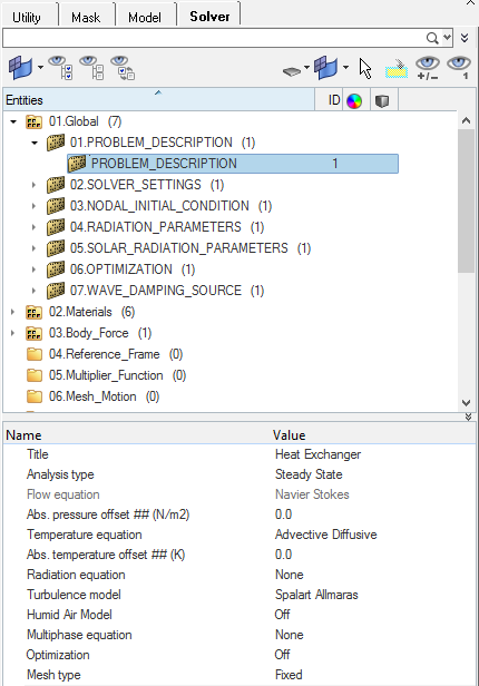
Figure 2.
Set Up Boundary Conditions and Assign Material Model Parameters
-
Click Fluid. In the Entity Editor,
- Change the Type to FLUID.
- Select Air_HM as the Material.
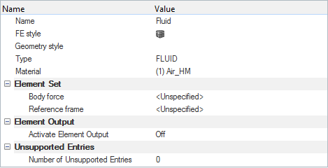
Figure 3. -
Click Inlet. In the Entity Editor,
- Change the Type to INFLOW.
- Change the Inflow velocity type to Cartesian and set the X velocity to 0.1 m/sec.
- Set the Temperature to 273 K.
- Change the Turbulence input type to Viscosity Ratio.
- For the Turbulent viscosity ratio, enter a value of 40.
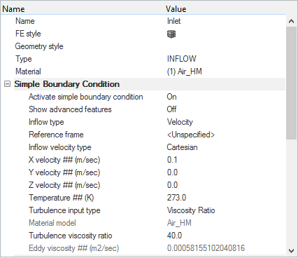
Figure 4. -
Click Outlet. In the Entity Editor, change the Type to OUTFLOW.
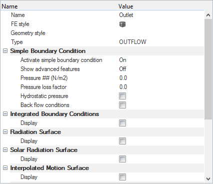
Figure 5. -
Click HEX_Inlet. In the Entity Editor,
- Change the Type to HEAT_EXCHANGER_COMPONENT.
- Verify that the Heat exchanger type is set to Constant Coolant Heat Reject.
- Set the Coolant Heat Reject to 200 W.
- Set the Coolant flow rate to 0.0006309 m3/sec.
- Set the Heat exchanger thickness to 0.06 m.
- Verify that the Upstream distance is set to 0.
- Change the Friction type to Kays London.
- Change the Core Friction Constant to 20.
- Change the Core Friction Exponent to -0.75.
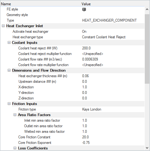
Figure 6. -
Click Walls. In the Entity Editor, verify that the Type is set to WALL.
The surface mesh elements on the external wall surfaces and interfaces can be grouped into one single collector. Auto_Wall, which is an advanced feature in AcuSolve, re-groups them into surface sets based on the element set they belong to and whether they are internal or external surfaces. This process is done internally without the user having to do it manually.
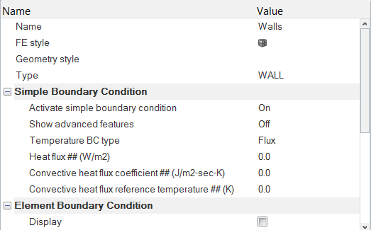
Figure 7.
Compute the Solution
In this step, you will launch AcuSolve directly from HyperMesh and compute the solution.
Run AcuSolve
-
Click
 on the ACU toolbar.
The Solver job Launcher dialog opens.
on the ACU toolbar.
The Solver job Launcher dialog opens. -
Leave the remaining options as
default and click Launch to start the solution
process.
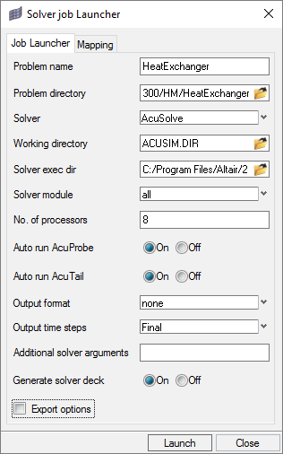
Figure 8.
Post-Process with AcuProbe
As the solution progresses, the AcuTail and AcuProbe windows are launched automatically. The surface output and residual ratios can be monitored using AcuProbe.
-
In the AcuProbe window, under the Data Tree, expand Residual Ratio,
right-click on Final, and select Plot
All.
Note: You might need to click
 on the toolbar in order to
properly display the plot.
on the toolbar in order to
properly display the plot.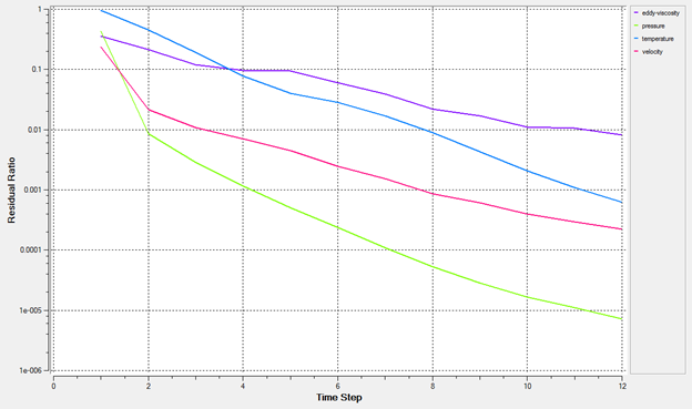
Figure 9. -
Click
 on the toolbar.
A User Function dialog opens.
on the toolbar.
A User Function dialog opens. -
On the next line, type value = Out - In.
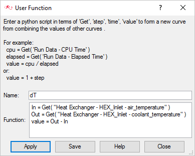
Figure 10.Note: The word “value” is case sensitive and should always be in lowercase characters. If it starts with a capital letter, it will give you an error window. -
Click Apply.
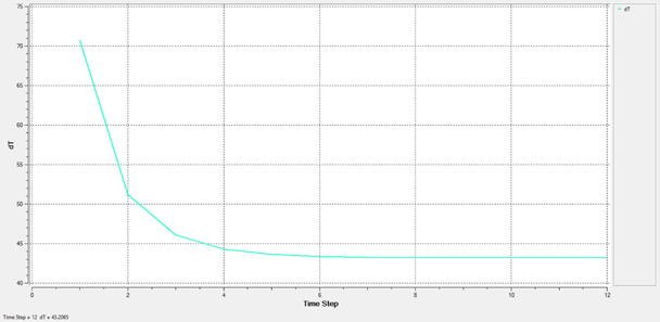
Figure 11.You can zoom into the plot by clicking
 and
then defining an area at the end of the curve. As shown in the figure below,
for the given problem, the temperature rise is 43.21 K.
and
then defining an area at the end of the curve. As shown in the figure below,
for the given problem, the temperature rise is 43.21 K.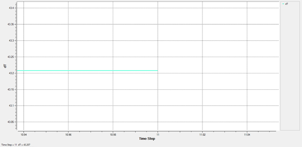
Figure 12.
Summary
In this tutorial, you successfully learned how to set up and solve a simulation involving a Heat Exchanger component. You imported the meshed geometry and then assigned the boundary conditions and material properties for all the regions. Once the solution was computed, you defined a user function in AcuProbe in order to create a plot of the temperature rise across the heat exchanger volume.