ACU-T: 3203 Heat Transfer Between Concentric Spheres – Discrete Ordinate Radiation Model
Prerequisites
This tutorial provides instructions for setting, solving and viewing results for a steady state simulation of radiation heat transfer between concentric spheres using the Discrete Ordinates Radiation model. Prior to starting this tutorial, you should have already run through the introductory HyperWorks tutorial, ACU-T: 1000 HyperWorks UI Introduction, and have a basic knowledge of HyperMesh, AcuSolve, and HyperView. To run this simulation, you will need access to a licensed version of HyperMesh and AcuSolve.
Prior to running through this tutorial, copy HyperMesh_tutorial_inputs.zip from <Altair_installation_directory>\hwcfdsolvers\acusolve\win64\model_files\tutorials\AcuSolve to a local directory. Extract ACU-T3203_DiscreteOrdinate.hm from HyperMesh_tutorial_inputs.zip.
Since the HyperMesh database (.hm file) contains meshed geometry, this tutorial does not include steps related to geometry import and mesh generation.
Problem Description
The problem to be addressed in this tutorial is shown schematically in Figure 1. In this problem, a DO radiation model is used to simulate the heat transfer due to radiation between concentric spheres. The inside surface of the inner and the outside surface of the outer sphere are both held at constant temperature while the gap between them radiates the heat from one sphere to the other.
The problem consists of a fluid region with arbitrary material properties between two concentric spheres with surfaces held at fixed temperature, as shown in the following figure, which is not drawn to scale. The radius of the outer sphere is 0.04 m and the radius of the inner sphere is 0.01 m. The inner surface of the inner sphere is defined to have a constant wall temperature at 300.0 K (26.85 ºC). The outer surface of the outer sphere is defined to have a constant wall temperature at 1300.0 K (1026.85 ºC). The fluid within the spheres is defined as a non-conducting material, allowing heat to transfer via radiation only.
The problem is solved as a steady state case to allow the heat transfer in the solid and fluid regions to reach an equilibrium.
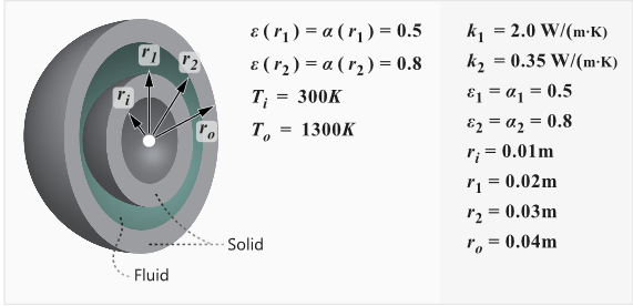
Figure 1.
Open the HyperMesh Model Database
-
Click the Open Model icon
 located on the standard toolbar.
The Open Model dialog opens.
located on the standard toolbar.
The Open Model dialog opens.
Set the General Simulation Parameters
-
Verify that the Radiation quadrature is set to S4.
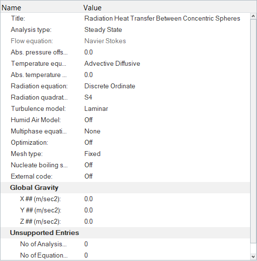
Figure 2. -
Turn off Flow and verify that the Temperature and Radiation fields are turned
On.
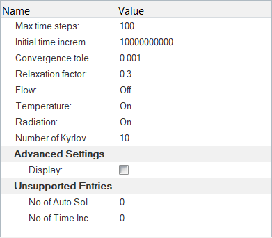
Figure 3.
Set Up Radiation Parameters and Boundary Conditions
In this step, you will define the radiation parameters i.e. emissivity models, surface boundary conditions for the problem, and assign material properties to the fluid and solid regions.
Set Up Material Model Parameters
-
Set the Absorption coefficient to 0.001.
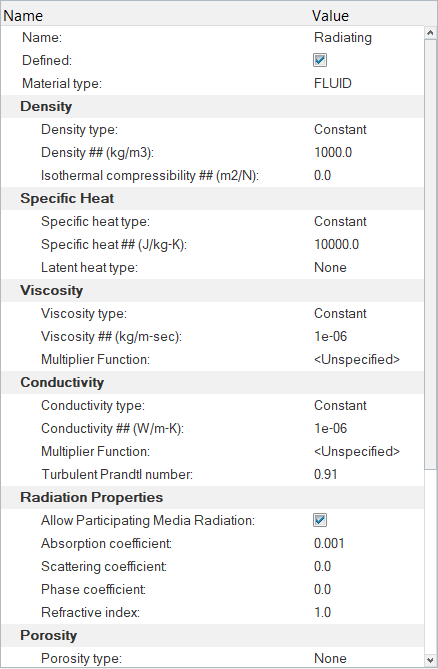
Figure 4.
Set Up Emissivity Model Parameters
-
In the Entity Editor, set the Emissivity to
0.5.
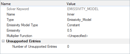
Figure 5.
Set Up Boundary Conditions
-
Click Radiating. In the Entity Editor, change the Type to
FLUID and set Radiating as the
Material.
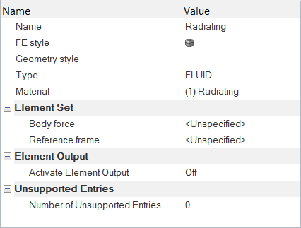
Figure 6. -
Click Inner. In the Entity Editor, change the Type to SOLID and set
Inner as the Material.

Figure 7. -
Click Outer. In the Entity Editor, change the Type to SOLID and set
Outer as the Material.
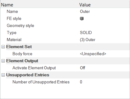
Figure 8. -
Click Inner_Inner_ri. In the Entity Editor,
- Verify that the Type is set to WALL.
- Change the Temperature BC type to Value.
- Set the Temperature to 300 K.
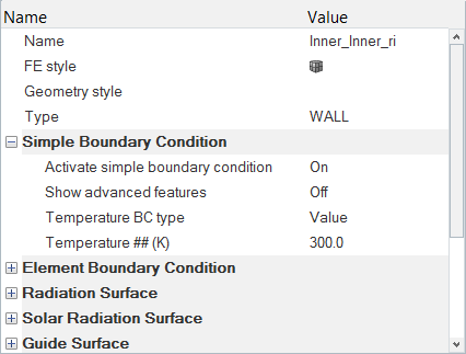
Figure 9. -
Click Outer_Outer_ro. In the Entity Editor,
- Verify that the Type is set to WALL.
- Change the Temperature BC type to Value.
- Set the Temperature to 1300 K.

Figure 10. -
Click Inner_Radiating_r1. In the Entity Editor,
- Verify that the Type is set to WALL.
- Change the Temperature BC type to Flux.
- Under the Radiation Surface tab, activate the Display check box and turn On the Activate radiation surface field.
- Verify that the Type is set to WALL and select Inner as the Emissivity model.
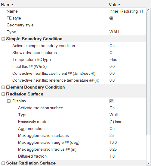
Figure 11. -
Click Outer_Radiating_r2. In the Entity Editor,
- Verify that the Type is set to WALL.
- Change the Temperature BC type to Flux.
- Under the Radiation Surface tab, activate the Display check box and turn On the Activate radiation surface field.
- Verify that the Type is set to WALL and select Outer as the Emissivity model.
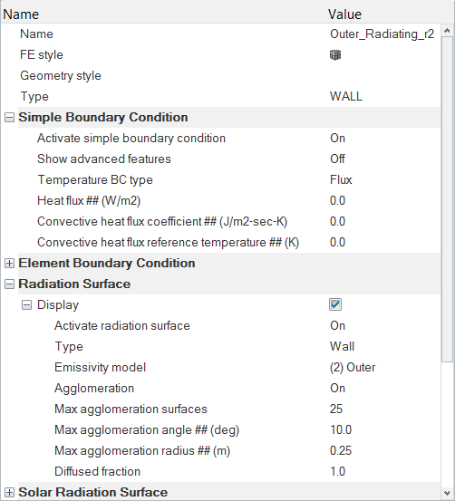
Figure 12.
Compute the Solution
In this step, you will launch AcuSolve directly from HyperMesh and compute the solution.
Run AcuSolve
-
Click
 on the ACU toolbar.
The Solver job Launcher dialog opens.
on the ACU toolbar.
The Solver job Launcher dialog opens. -
Leave the remaining options as
default and click Launch to start the solution
process.
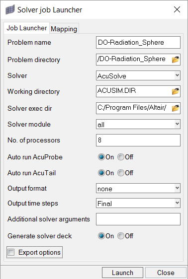
Figure 13.
Post-Process the Results with HyperView
Open HyperView and Load the Model and Results
-
In the Load model and results panel, click
 next
to Load model.
next
to Load model.
Create Temperature Contours
In this step, you will create a contour plot of temperature distribution across the domain.
-
Click
 on the Results toolbar to open the Contour panel.
-
In the panel area, under the Display tab, turn off
the Discrete color option.
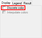
Figure 14. -
Click
 beside
Section 1 to turn off the grid display in the graphics window.
beside
Section 1 to turn off the grid display in the graphics window.
-
Orient the display to the xz-plane by clicking
 on the Standard Views toolbar.
-
Verify that the contour plot looks like the figure below.
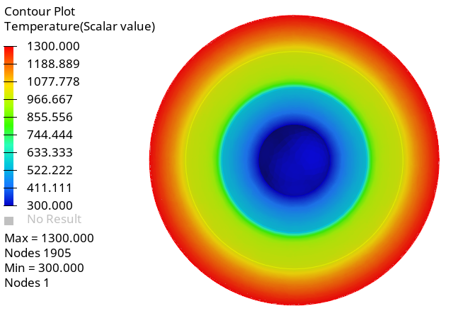
Figure 15.
Summary
In this tutorial, you worked through a workflow to set-up a DO-Radiation model, carry out a radiation heat transfer simulation, and post-process the results using HyperWorks products, namely AcuSolve, HyperMesh, and HyperView. You started by importing the model in Altair HyperMesh. Then you defined the simulation parameters and launched AcuSolve directly from within HyperMesh. Upon completion of the solution by AcuSolve, you used HyperView to post-process the results and create contour plots.