ACU-T: 3100 Conjugate Heat Transfer in a Mixing Elbow
This tutorial provides the instructions for setting up, solving, and viewing results for a simulation of 3D turbulent-flow with conjugate heat transfer in a mixing elbow. It is designed to introduce you to the AcuSolve tool set with a simple problem.
- Simulating heat transfer within a fluid
- Simulating heat transfer between a fluid and a solid (conjugate heat transfer)
- Creation of a new material model
- Modeling of surfaces shared between solid and fluid volumes
- Propagation (copying) of settings from one surface group to another
Prerequisites
You should have already run through the introductory tutorial, ACU-T: 2000 Turbulent Flow in a Mixing Elbow. It is assumed that you have some familiarity with AcuConsole, AcuSolve, and AcuFieldView. You will also need access to a licensed version of AcuSolve.
Prior to running through this tutorial, copy AcuConsole_tutorial_inputs.zip from <Altair_installation_directory>\hwcfdsolvers\acusolve\win64\model_files\tutorials\AcuSolve to a local directory. Extract mixingElbowHeat.x_t from AcuConsole_tutorial_inputs.zip.
Analyze the Problem
An important first step in any CFD simulation is to examine the engineering problem to be analyzed and determine the settings that need to be provided to AcuSolve. Settings can be based on geometrical components (such as volumes, inlets, outlets, or walls) and on flow conditions (such as fluid properties, velocity, or whether the flow should be modeled as turbulent or as laminar).
The problem to be addressed in this tutorial is shown schematically in Figure 1. It consists of a mixing elbow made of stainless steel with water entering through two inlets with different velocities and with different temperatures. The geometry is symmetric about the XY midplane of the pipe, as shown in the figure. This symmetry allows the flow to be modeled with the use of a symmetry plane. The use of a symmetry plane leads to reduced computation time while still providing an accurate solution.

Figure 1. Schematic of Mixing Elbow with Stainless-steel Walls
Details of the problem characteristics are shown in the following images extracted from a sample worksheet that was created prior to setting up the case for AcuSolve.
The diameter of the large inlet is 0.1 m, the inlet velocity (v) is 0.4 m/s and the temperature (T) of the fluid entering the large inlet is 295 K. The diameter of the small inlet is .025 m, the velocity is 1.2 m/s, and the temperature of the fluid entering the small inlet is 320 K. The pipe wall has a thickness of 0.005 m.
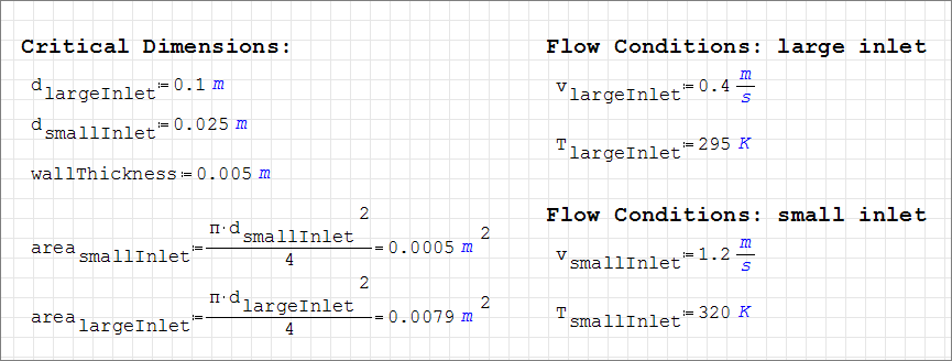
Figure 2.
The fluid in this problem is water, with the following properties that do not change with temperature; a density (ρ) of 1000 kg/m3, a molecular viscosity (μ) of 1 X 10⁻³ kg/m-sec, a conductivity (k) of 0.598 W/m-K, and a specific heat (cp) of 4183 J/kg-K, as shown in the worksheet.
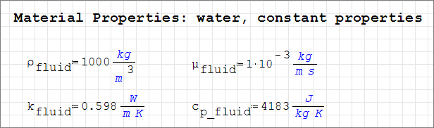
Figure 3.
The pipe walls are made of stainless steel with a density of 8030 kg/m3, a conductivity of 16.2 W/m-K, and a specific heat of 500 J/kg-K.
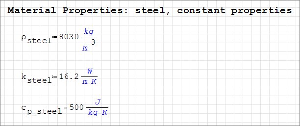
Figure 4.
Based on mass conservation, the combined flow rate (Q) yields a velocity of 0.475 m/s downstream of the small inlet. This value is useful in determining the Reynolds number, which in turn can be used to determine if the flow should be modeled as turbulent, or if it should be modeled as laminar.
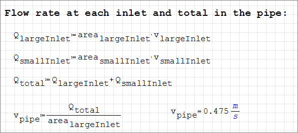
Figure 5.
The Reynolds numbers of 40,000 at the large inlet, 30,000 at the small inlet, and 47,500 for the combined flow indicate that the flow is turbulent throughout the flow domain.
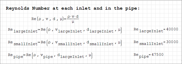
Figure 6.
The simulation will be set up to model steady state, turbulent flow with varying temperature. In addition, the thermal characteristics of the flow will be modeled using advection and diffusion equations.
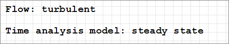
Figure 7.
In addition to setting appropriate conditions to capture the physics of the simulation, it is important to generate a mesh that is sufficiently refined to provide good results. In this tutorial the global mesh size is set to provide at least 30 mesh elements around the circumference of the large inlet. For this problem, the global mesh size is 0.0106 m. This mesh size was chosen to provide a quick turnaround time for the model. For real-world simulations, you would modify your mesh settings after an initial solution until a mesh-independent solution is reached (that is, a solution that does not change with further mesh refinement).
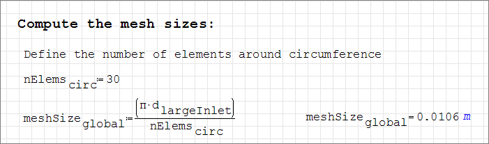
Figure 8.
AcuSolve allows for mesh refinements in a user-defined region that is independent of geometric components of the problem such as volumes, model surfaces, or edges. It is useful to refine the mesh in areas where gradients in pressure, velocity, eddy viscosity, and the like are steep. For this problem, the flow entering the large pipe from the side pipe creates large velocity gradients that need to be resolved. A mesh refinement zone is used to capture the flow in this region.
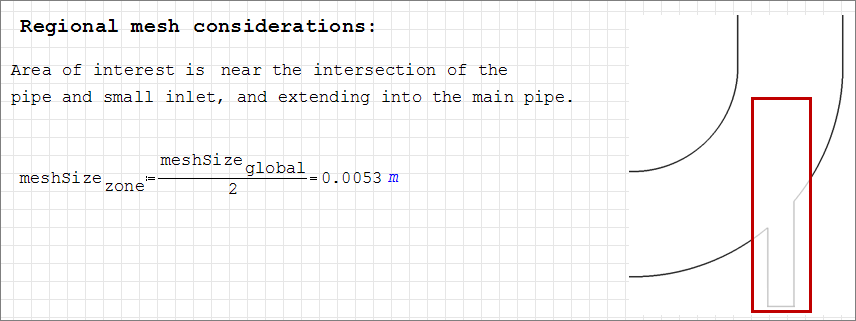
Figure 9.
Once a solution is calculated, the flow properties of interest are the steady state temperature contours on the symmetry plane, velocity vectors on the symmetry plane, temperature contours on the pipe walls, and temperature contours at the pipe outlet.
Define the Simulation Parameters
Start AcuConsole and Create the Simulation Database
In this tutorial, you will begin by creating a database, populating the geometry-independent settings, loading the geometry, creating groups, setting group attributes, adding geometry components to groups, and assigning mesh controls and boundary conditions to the groups. Next you will generate a mesh and run AcuSolve to converge on a steady state solution. Finally, you will visualize the results using AcuFieldView.
In the next steps you will start AcuConsole, create the database for storage of AcuConsole settings and set the location for saving mesh and solution information for AcuSolve.
-
Click the File menu, then click
New to open the New data
base dialog.
Note: You can also open the New data base dialog by clicking
 on the toolbar.
Set General Simulation Parameters
In the next steps you will set parameters that apply globally to the simulation. To simplify this task, you will use the BAS filter in the Data Tree Manager. The BAS filter limits the options in the Data Tree to show only the basic settings.
The general parameters that you will set for this tutorial are for turbulent flow, steady state time analysis and for thermal analysis using advection-diffusion equations.
-
Click BAS in the Data Tree Manager to switch to basic view in the Data Tree.
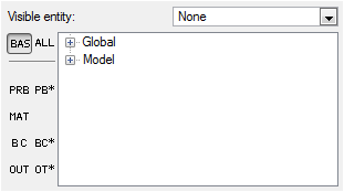
Figure 10. -
Double-click the Global
Data Tree item to expand it.
Tip: You can also expand a tree item by clicking
 next to the item name.
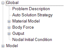
Figure 11. -
Set the Turbulence equation to Spalart
Allmaras.
The robustness and accuracy of the Spalart-Allmaras turbulence model makes it an excellent choice for simulation of steady state flows.
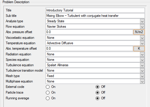
Figure 12.
Set Solution Strategy Parameters
In the next steps you will set the parameters that control the behavior of AcuSolve as it progresses during the solution.
-
Enter 0.4 for the Relaxation
factor.
The relaxation factor is used to improve convergence of the solution. Typically a value between 0.2 and 0.4 provides a good balance between achieving a smooth progression of the solution and the extra compute time needed to reach convergence. Higher relaxation factors cause AcuSolve to take more time steps to reach a steady state solution. A high relaxation factor is sometimes necessary in order to achieve convergence for very complex applications.
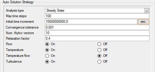
Figure 13.
Set Material Model Parameters
AcuConsole has three pre-defined materials, Air, Aluminum and Water.
In the next steps you will verify that the pre-defined material properties of water match the desired properties for this problem. You will also create a new material, stainless steel, and set the desired material properties.
Figure 14.
-
Create a new material model for stainless steel.
Figure 15.- Right-click Material Model in the Data Tree.
- Click New.
-
Save the database to create a backup of your settings.
This can be achieved with any of the following methods.
- Click the File menu, then click Save.
- Click
 on
the toolbar.
on
the toolbar. - Click Ctrl+S.
Note: Changes made in AcuConsole are saved into the database file (*.acs) as they are made. A save operation copies the database to a backup file, which can be used to reload the database from that saved state in the event that you do not want to commit future changes.
Import the Geometry and Define the Model
Import the Geometry
-
Select mixingElbowHeat.x_t and click
Open to open the Import Geometry
dialog.
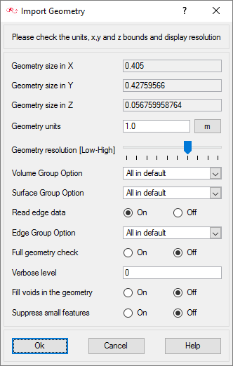
Figure 16.For this tutorial, the default values for the Import Geometry dialog are used to load the geometry. If you have previously used AcuConsole, be sure that any settings that you might have altered are manually changed to match the default values shown in the figure. With the default settings, volumes from the CAD model are added to a default volume group. Surfaces from the CAD model are added to a default surface group. You will work with groups later in this tutorial to create new groups, set flow parameters, add geometric components, and set meshing parameters.
-
Click Ok to complete
the geometry import.

Figure 17.The color of objects shown in the modeling window in this tutorial and those displayed on your screen may differ. The default color scheme in AcuConsole is "random," in which colors are randomly assigned to groups as they are created. In addition, this tutorial was developed on Windows. If you are running this tutorial on a different operating system, you may notice a slight difference between the images displayed on your screen and the images shown in the tutorial.
Create a Volume Group and Apply Volume Parameters
Volume groups are containers used for storing information about volumes. This information includes the list of geometric volumes associated with the container, as well as parameters such as material models and mesh sizing information.
When the geometry was imported into AcuConsole, all volumes were placed into the "default" volume container.
In the next steps you will create a new group for the steel wall volume; set the material for that group; add the volumes from the geometry to that volume group; rename the default volume group to Fluid and set the material for that group; then add the volumes from the geometry to that group.
-
Toggle the display of the default volume container by clicking
 and
and
 next to the volume name.
Note: You may not see any change when toggling the display if Surfaces are being displayed, as surfaces and volumes may overlap.
next to the volume name.
Note: You may not see any change when toggling the display if Surfaces are being displayed, as surfaces and volumes may overlap. -
Set the material model for the volume to use the Stainless Steel.
- Expand the Steel Walls volume in the tree.
- Double-click Element Set to open the Element Set detail panel.
- Change the Medium to Solid to define this volume as a solid.
- For Material model, click Stainless Steel.
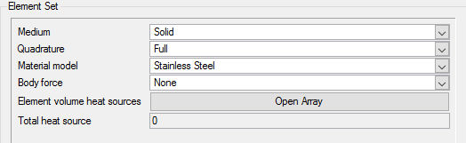
Figure 18. -
Add the pipe wall components in the geometry to this volume group.
-
Click the outer surface of the pipe wall.
If you rotate the view, by Ctrl + left-clicking, you can see that only the outer volume is highlighted.
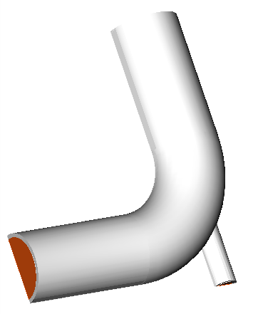
Figure 19.
-
Click the outer surface of the pipe wall.
-
Set the material model used for the fluid in the
simulation.
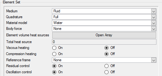
Figure 20.
Create Surface Groups and Apply Surface Attributes
Surface groups are containers used for storing information about a surface. This information includes the list of geometric surfaces associated with the container, as well as attributes such as boundary conditions, surface outputs, and mesh sizing information.
In the next steps you will define surface groups, assign the appropriate attributes for each group in the problem, and add surfaces to the groups.
Set Inflow Boundary Conditions for the Large Inlet
In the next steps you will define a surface group for the large inlet, set the inlet velocity, and add the main inlet from the geometry to the surface group.
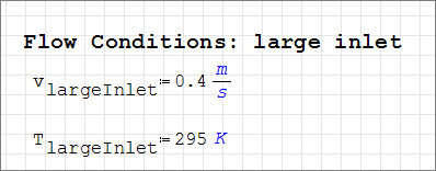
Figure 21.
-
Set the Temperature to 295 K.
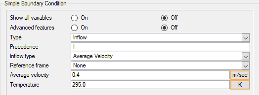
Figure 22. -
Add a geometry surface to the Large Inlet
group.
-
Click on the large inlet face.
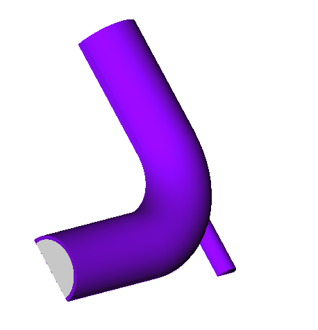
Figure 23.At this point, the inlet should be highlighted.
-
Click on the large inlet face.
Set Inflow Boundary Conditions for the Small Inlet
In the next steps you will define a surface group for the small inlet, assign the appropriate attributes, and add the small inlet from the geometry to the surface group.
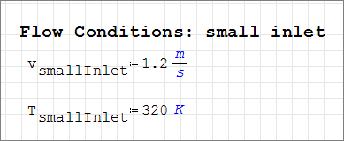
Figure 24.
-
Set the Temperature to 320 K.
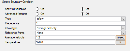
Figure 25. -
Add a geometry surface to the Small Inlet
group.
-
Rotate the model to expose the small inlet by Ctrl+left-clicking near the bottom of the geometry
and moving the cursor toward the top of the window.
Note: If you need to zoom in or out, Ctrl+right-click and drag the cursor down or up. You can also restore the initial view by clicking
 .
. -
Left-click on the small inlet face.
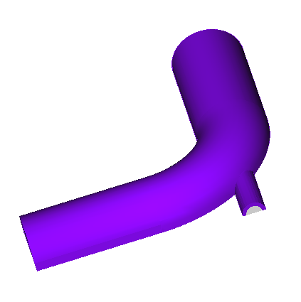
Figure 26.At this point, the small inlet should be highlighted.
-
Rotate the model to expose the small inlet by Ctrl+left-clicking near the bottom of the geometry
and moving the cursor toward the top of the window.
Set Outflow Boundary Conditions for the Outlet
In the next steps you will define a surface group for the outlet, assign the appropriate attributes and add the outlet from the geometry to the surface group.
-
Change the Type to
Outflow.
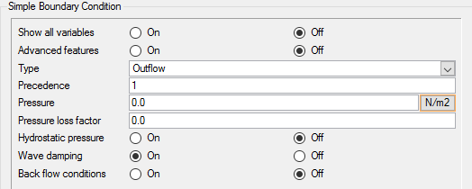
Figure 27. -
Add a geometry surface to the Outlet surface
container.
-
Click on the outlet face.
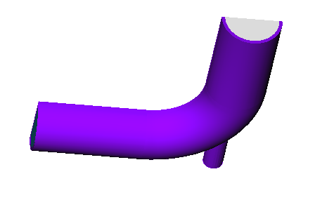
Figure 28.At this point, the outlet should be highlighted.
-
Click on the outlet face.
Set Wall Boundary Conditions for the Steel Pipe Outer Walls
In the next steps you will define a surface group for the steel pipe outer walls, assign the appropriate attributes and add the pipe walls from the geometry to the surface group. In this simulation, you will not be modeling the air surrounding the pipe. However, you will specify a convective heat transfer coefficient and reference temperature to account for heat transfer from the pipe walls to the surroundings.
-
Enter 302.594 for the Convective heat flux reference
temperature and verify that the units are K.
This temperature value specifies that the surroundings of the pipe are at a constant temperature of 302.594 K.
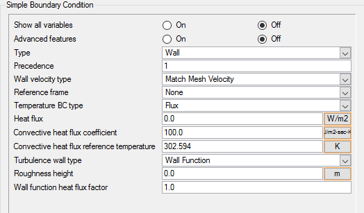
Figure 29. -
Add a geometry surface to the Steel Pipe - Outer Walls group.
-
Right-click Steel Pipe - Outer Walls and click
Add to.
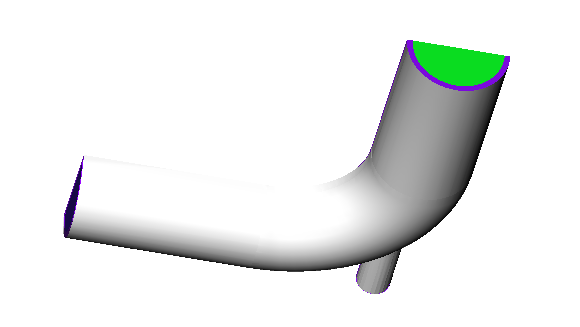
Figure 30.At this point, the outer pipe walls should be highlighted.
-
Right-click Steel Pipe - Outer Walls and click
Add to.
Set Boundary Conditions for the Steel Pipe Inner Walls
In the next steps you will define a surface group for the steel pipe inner wall, assign the appropriate attributes, and add the pipe walls from the geometry to the surface group.
-
Turn off the display of the Steel Pipe - Outer Walls.
- Click next to the
surface so that it is in the display off state (),
or,
- Right-click Steel Pipe - Outer Walls in the tree, and click Display off.
Turning off the display of the outer walls will make it easier to add geometric surfaces to the inner wall group. - Click
-
Add geometry surfaces to the Steel Pipe - Inner Walls group.
-
Click the pipe near the main inlet, the pipe near the elbow, the pipe
near the outlet, and the pipe near the side inlet to select the four
surfaces that make up the inner surface of the steel pipe wall.
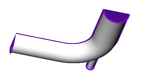
Figure 31.At this point, the inner walls of the steel pipe should be highlighted.
-
Click the pipe near the main inlet, the pipe near the elbow, the pipe
near the outlet, and the pipe near the side inlet to select the four
surfaces that make up the inner surface of the steel pipe wall.
Set Wall Boundary Conditions for the Large Pipe
In the next steps you will define a surface group for the pipe walls, assign the appropriate attributes, and add the elbow pipe walls from the geometry to the surface group.
-
Add geometry surfaces to this group.
-
Click on the pipe near the large
inlet, the pipe near the elbow, and the pipe near the outlet to select
the three surfaces that make up the main pipe wall.
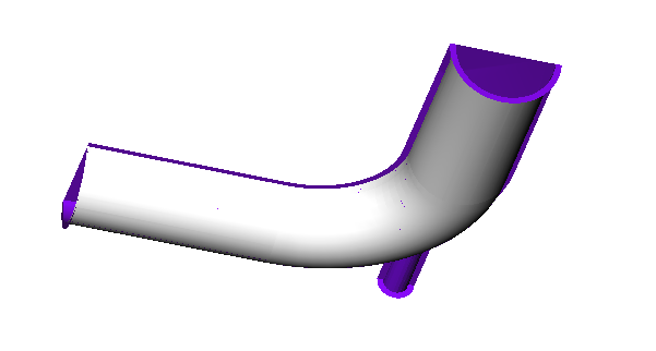
Figure 32.At this point, the pipe walls should be highlighted.
-
Click on the pipe near the large
inlet, the pipe near the elbow, and the pipe near the outlet to select
the three surfaces that make up the main pipe wall.
Set Wall Boundary Conditions for the Small Pipe
In the next steps you will define a surface group for the side pipe wall, assign the appropriate parameters, and add the side pipe wall from the geometry to the surface group.
-
Add geometry surfaces to this group.
-
Click on the pipe near the side inlet.
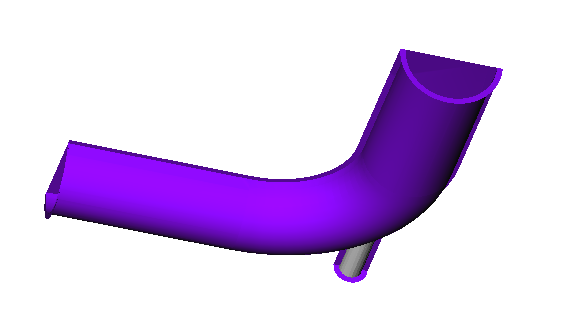
Figure 33.At this point, the side pipe wall should be highlighted.
-
Click on the pipe near the side inlet.
Set Symmetry Boundary Conditions for the Pipe Symmetry Plane
This geometry is symmetric about the XY midplane, and can therefore be modeled with half of the geometry. In order to take advantage of this, the midplane needs to be identified as a symmetry plane. The symmetry boundary condition enforces constraints such that the flow field from one side of the plane is a mirror image of that on the other side.
In the next steps you will create a surface group for the symmetry plane of the pipe, assign the appropriate attributes, and add the side pipe wall from the geometry to the surface group.- Create a new surface group and rename it to Symmetry.
- Expand the Symmetry surface in the tree.
- Double-click Simple Boundary Condition under Symmetry to open the Simple Boundary Condition detail panel.
- Change the Type to Symmetry.
- Turn off the display of all surface items except Symmetry and default.
-
Add geometric faces to this group.
-
Click on the Symmetry plane.
Figure 34.At this point, the symmetry plane should be highlighted.
-
Click on the Symmetry plane.
Set Boundary Conditions for the Steel Pipe Ends
In the next steps you will define a surface group for the ends of the steel pipe, assign the appropriate attributes, and add the pipe ends from the geometry to the surface group.
-
Add geometric faces to this group.
-
Click on the pipe ends at the large inlet, the small inlet, and the
outlet.
Note: You may need to rotate the graphic to see that the pipe end at the large inlet is highlighted.
Figure 35.At this point, the pipe ends should be highlighted.
-
Click on the pipe ends at the large inlet, the small inlet, and the
outlet.
Set Symmetry Boundary Conditions for the Steel Pipe Symmetry Plane
- Rename the default surface group to Steel Pipe - Symmetry.
- Expand the Steel Pipe - Symmetry surface in the tree.
- Double-click Simple Boundary Condition under Steel Pipe - Symmetry to open the Simple Boundary Condition detail panel.
- Change the Type to Symmetry.
- Save the database to create a backup of your settings.
Assign Mesh Controls
Set Global Meshing Parameters
Now that the simulation has been defined, parameters need to be added to define the mesh sizes that will be created by the mesher.
- Global mesh controls apply to the whole model without being tied to any geometric component of the model.
- Zone mesh controls apply to a defined region of the model, but are not associated with a particular geometric component.
- Geometric mesh controls are applied to a specific geometric component. These controls can be applied to volume groups, surface groups, or edge groups.
In the next steps you will set global meshing parameters. In subsequent steps you will create zone and surface meshing parameters.
Figure 36.
-
Turn off the Curvature refinement parameters option.
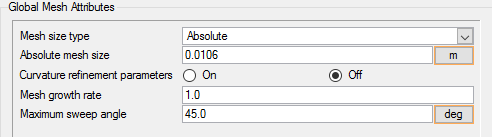
Figure 37.
Set Zone Meshing Parameters
In addition to setting meshing characteristics for the whole problem, you can assign meshing parameters to a zone within the problem where you want to be able to resolve flow with a mesh that is more refined than the global mesh. A zone mesh refinement can be created using basic shapes to control the mesh size within that shape. These types of mesh refinement are used when refinement is needed in an area that does not correspond to a geometric item.
In the next steps you will define mesh controls for a region around the small pipe and extending into the main pipe by using a zone mesh control. The region of interest for this refinement is a cylinder that encloses the small pipe and extends into the main pipe.
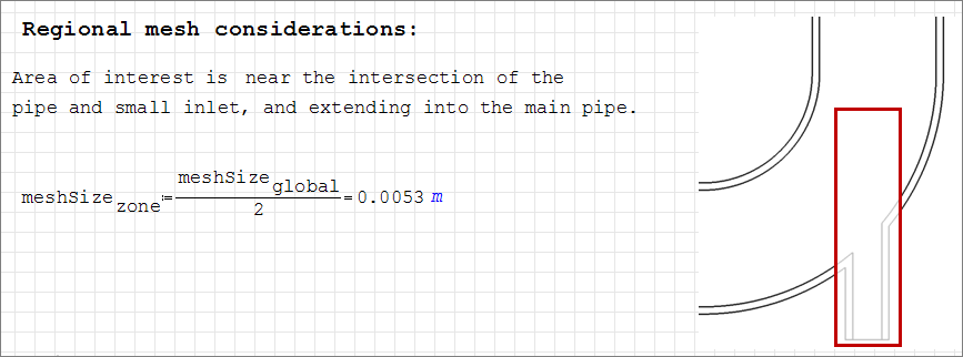
Figure 38.
-
Restore the initial view by clicking on
the View Manager toolbar.
-
Enter 0.0053 m
for the Mesh size.
This will result in a zone where the mesh size is half of the mesh size in the rest of the pipe.
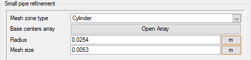
Figure 39.Note: When setting mesh size for refinement zones, the best practice is to choose a value that is the global mesh size divided by a power of 2, that is, 1/2, 1/4, 1/8, and the like. -
Set the location of the mesh refinement by
defining the center points of the end faces of the cylinder.
-
Click OK.
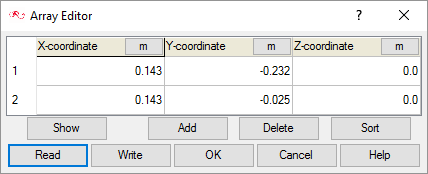
Figure 40.
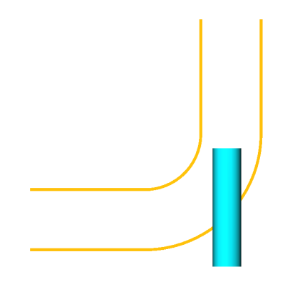
Figure 41. -
Click OK.
Set Meshing Attributes for Surface Groups
In the following steps you will set meshing attributes that will allow for localized control of the mesh size on surface groups that you created earlier in this tutorial. Specifically, you will set local meshing attributes that control the growth of boundary layer elements normal to the surfaces of the main pipe and of the side pipe.
Set Meshing Parameters for the Large Pipe
-
Enter 4 for the Number of layers.
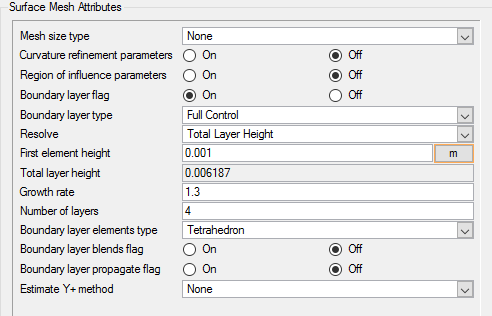
Figure 42.
Propagate Meshing Parameters to the Small Pipe
The local mesh settings for the small pipe are the same as for the large pipe. AcuConsole has the capability to propagate, or "copy and paste," settings from one group to another. In the following steps you will propagate the local mesh settings from the large pipe surface group to the small pipe surface group.
-
Scroll down the list of surfaces and click Small
Pipe.
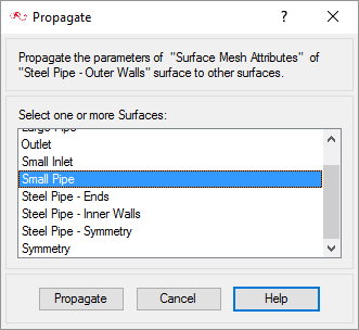
Figure 43.
Set Meshing Parameters for the Steel Pipe Outer Walls
In the following steps you will set meshing parameters that will allow for localized control of the mesh size near the outer walls of the steel pipe.
-
Enter 1 for the Number of layers.
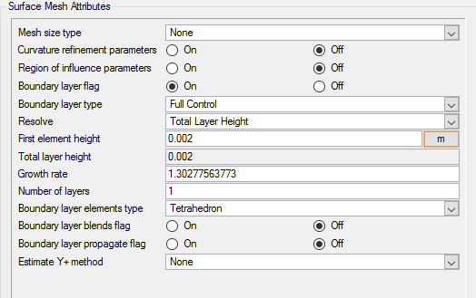
Figure 44.
Propagate Meshing Attributes to the Steel Pipe Inner Walls
The local mesh settings for the inner walls of the pipe are the same as for the outer walls. In the following steps you will propagate the local mesh settings from the surface group containing the steel pipe outer walls to the surface group containing the steel pipe inner walls.
Generate the Mesh
In the next steps you will generate the mesh that will be used when computing a solution for the problem.
-
Click
 on the toolbar to open the Launch
AcuMeshSim dialog.
on the toolbar to open the Launch
AcuMeshSim dialog.
-
Click Ok to begin
meshing.
During meshing an AcuTail window opens. Meshing progress is reported in this window. A summary of the meshing process indicates that the mesh has been generated.
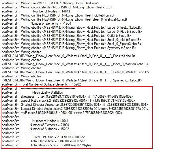
Figure 45. -
Turn off the display of small pipe refinement under by clicking next to the surface so that it is in the display off
state ().
Details of the mesh on the side pipe are shown in Figure 46. This view was obtained by turning off the display of all surfaces except Symmetry and Steel Pipe - Symmetry, then zooming in on the region where the small pipe joins the large pipe.
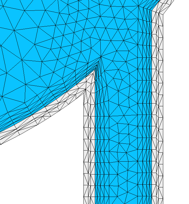
Figure 46. Mesh Details Around the Pipe Intersection Viewed on the Symmetry PlaneNote that the mesh size in the main pipe decreases from left to right in the transition from a region where global settings determine the size to the zone around the small pipe where the settings are for a finer mesh.
Compute the Solution and Review the Results
Run AcuSolve
In the next steps you will launch AcuSolve to compute the solution for this case.
-
Click
 on the toolbar to open the
Launch AcuSolve dialog.
on the toolbar to open the
Launch AcuSolve dialog.
For this case, the default values will be used.
Based on these settings, AcuConsole will generate the AcuSolve input files, then launch the solver. AcuSolve will run using four processors to calculate the steady state solution for this problem.
-
Click Ok to start the
solution process.
While computing the solution, an AcuTail window opens. Solution progress is reported in this window. A summary of the solution process indicates that the run has been completed.
The information provided in the summary is based on the number of processors used by AcuSolve. If you use a different number of processors than indicated in this tutorial, the summary for your run may be slightly different than the summary shown.
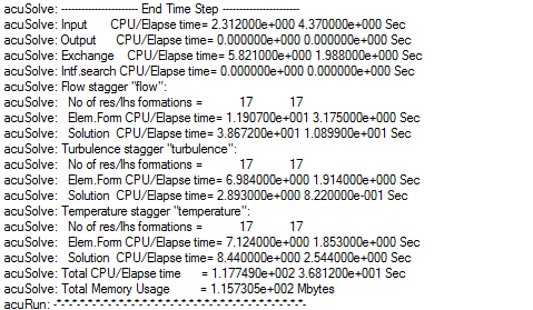
Figure 47.
View Results with AcuFieldView
Now that a solution has been calculated, you are ready to view the flow field using AcuFieldView. AcuFieldView is a third-party post-processing tool that is tightly integrated toAcuSolve. AcuFieldView can be started directly from AcuConsole, or it can be started from the Start menu, or from a command line. In this tutorial you will start AcuFieldView from AcuConsole after the solution is calculated by AcuSolve.
In the next steps you will start AcuFieldView, manipulate the view of the model, display temperature contours and velocity vectors on the symmetry plane, display temperature contours on the pipe wall symmetry plane and display temperature contours at the outlet.
Start AcuFieldView
-
Click
 on the
AcuConsole toolbar to open the
Launch AcuFieldView dialog.
on the
AcuConsole toolbar to open the
Launch AcuFieldView dialog.
Manipulate the Model View in AcuFieldView
When AcuFieldView is started directly from AcuConsole, the model will be displayed in an isometric view with a Boundary Surface dialog open. The initial view is shown in perspective, with an outline around the model. You will manipulate the view in the next steps, and in later steps will view different flow characteristics using the Boundary Surface dialog.
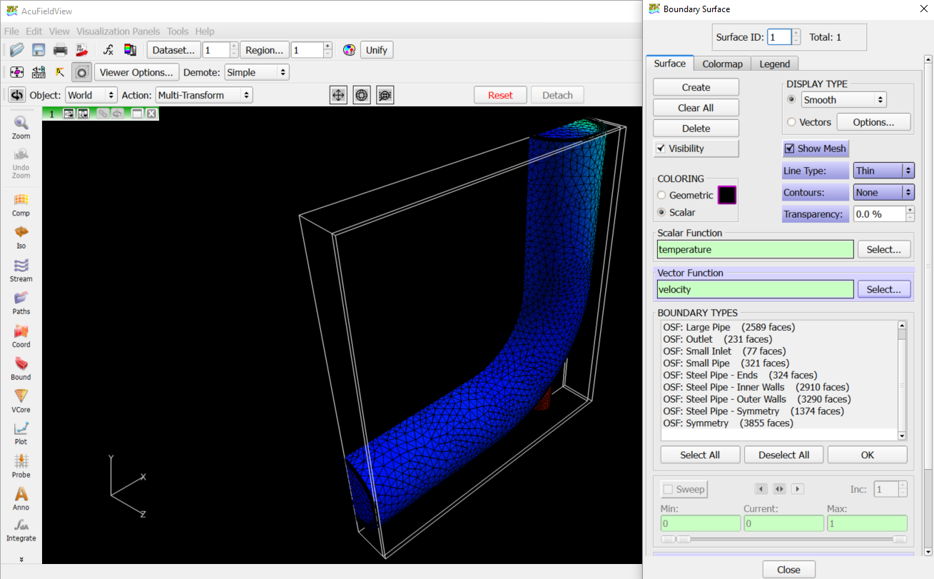
Figure 48.
-
Change the background color to white.
-
Click the white swatch, then click Close.
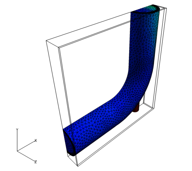
Figure 49.
-
Click the white swatch, then click Close.
-
Turn off the display of the outline around the model by clicking
 on
the toolbar.
on
the toolbar.
-
Change the view from perspective to orthographic.
- Click on the View menu.
- Click Perspective to disable this option.
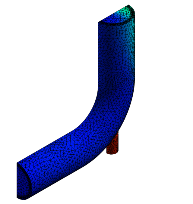
Figure 50. -
Orient the model to view it from the positive Z direction (+Z).
-
Click
 on the toolbar to open the Defined
Views dialog.
on the toolbar to open the Defined
Views dialog.
-
Click
 .
.
You will see the view change as soon as you click a button in the Defined Views dialog.
You can move, zoom, and rotate the view in AcuFieldView in a similar fashion as in AcuConsole. AcuFieldView uses a different mapping for mouse-button actions.
Action Mouse Button move (pan) left rotate middle zoom right -
Click
Display Contours of Fluid Temperature on the Symmetry Plane
In the next steps you will create a boundary surface to display contours of fluid temperature on the symmetry plane.
-
Click
 to open the Boundary
Surface dialog.
Note: The dialog may already be open. This step will put the focus on the dialog.
to open the Boundary
Surface dialog.
Note: The dialog may already be open. This step will put the focus on the dialog. -
Set the symmetry plane as the location for
display of the contours.
- Click OSF: Symmetry in the list of Boundary Types.
- Click OK.
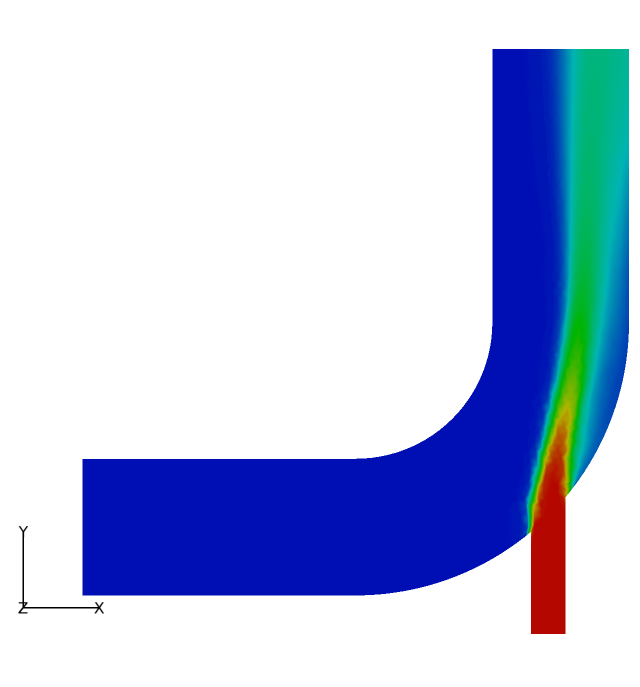
Figure 51. -
Add a legend to the view.
- Click the Legend tab in the Boundary Surface dialog.
- Enable the Show Legend option.
- Enable the Frame option.
- Click the white color swatch next to Geometric in the Color group and set the color for the legend values to black.
- Click the white color swatch next to the Title field and set the color for the title to black.
- Move the legend by Shift+left-clicking and dragging the legend to the left.
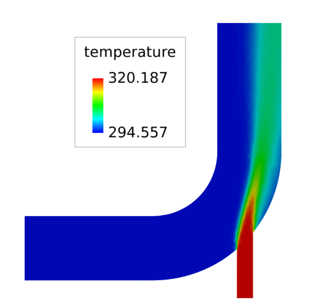
Figure 52.
Add Velocity Vectors to the View
In the next steps you will create a new boundary surface and display velocity vectors on that surface.
-
Set vector options.
-
Enable the Skip option
and set it to 37.5%.
The Skip option determines the percentage of vectors to skip from being displayed. The setting of 37.5% will result in 62.5% of the vectors being displayed.
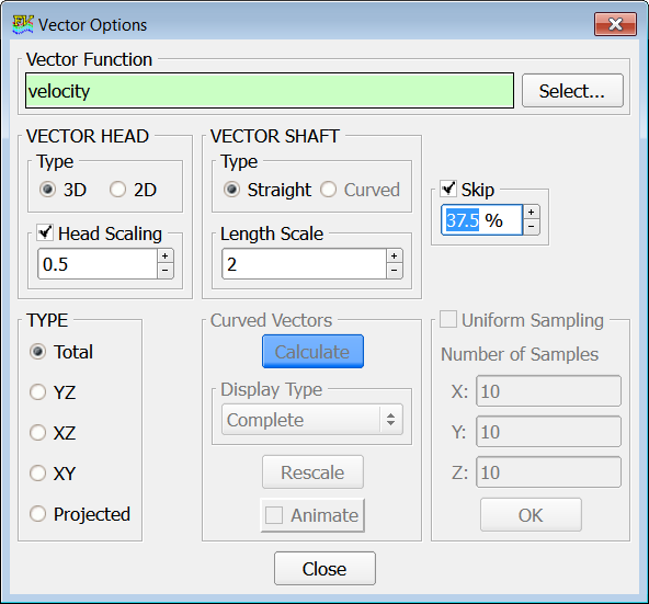
Figure 53.
-
Enable the Skip option
and set it to 37.5%.
-
Set the symmetry plane as the location for
display of the vectors.
- Click OSF: Symmetry in the list of Boundary Types.
- Click OK.
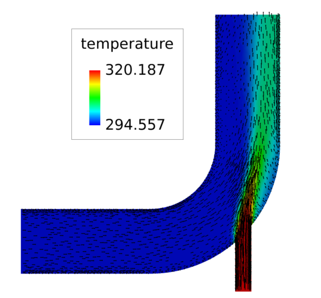
Figure 54. -
Zoom in on the junction of the small inlet with the
main pipe to view details of velocity vectors.
-
Click
 on the toolbar.
- Draw a box around the junction of the two pipes.
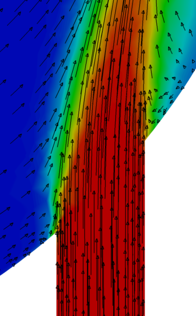
Figure 55.Note: The Show Legend option for the temperature contour (Surface ID 1) is disabled in order to capture this image.The velocity vectors indicate the direction of flow. The vector length indicates the magnitude of the flow velocity. Adding velocity vectors to a view with temperature contours allows you to visualize temperature and velocity simultaneously. -
Click
Display Contours of Temperature on the Steel Pipe Walls
In the next steps you will create a boundary surface to display contours of temperature on the stainless steel pipe walls at the symmetry plane.
-
Click
 on the Transform Controls toolbar to center the visible
surfaces and to fit the view in the window.
on the Transform Controls toolbar to center the visible
surfaces and to fit the view in the window.
-
Click to open the Boundary
Surface dialog.
Note: The dialog may already be open. This step will put the focus on the dialog.
-
Set the stainless-steel pipe symmetry plane as the location for display of the
contours.
- Scroll up in the list of Boundary Types and click OSF:Steel Pipe - Symmetry.
- Click OK.
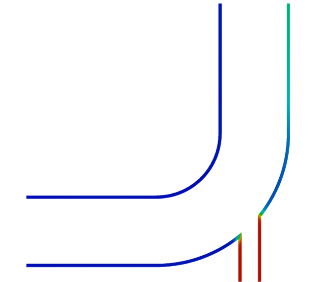
Figure 56.
Display Contours of Temperature at the Outlet
In the next steps you will create a boundary surface to display contours of temperature at the outlet.
-
Click to open the Boundary
Surface dialog.
-
Orient the view so that you can see the contours on the outlet.
-
Click on the Transform Controls toolbar.
- Set the Viewing Direction to -Y.
-
Click on the Transform Controls
toolbar to center the visible surfaces and to fit the view in the
window.
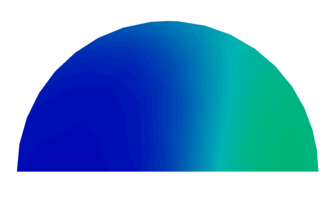
Figure 57. -
Click
-
Change the color scale to better resolve differences in the temperature
contours.
When the scalar function for temperature is calculated by AcuFieldView, minimum and maximum values are calculated for use in a colormap for the contour display. You can edit the coloring to better resolve differences in the pressure distribution.
-
Click the Colormap
tab.
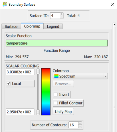
Figure 58.Notice that the Min: and Max: values for the Function Range change when the Local option is toggled.
-
Enable the Local option.
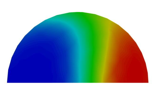
Figure 59.
-
Click the Colormap
tab.
Summary
In this tutorial, you worked through a basic workflow to set up a simulation of conjugate heat transfer in a mixing elbow. Once the case was set up, you generated a mesh and generated a solution using AcuSolve. Results were post-processed in AcuFieldView to allow you to create contour and vector views along the symmetry plane of the model. New features introduced in this tutorial include: flows of different temperatures, simulating heat transfer within a fluid, simulating heat transfer between a fluid and a solid (conjugate heat transfer), creation of a new material model, modeling of shared surfaces at fluid/solid interfaces, and copying and pasting (propagation) of settings from one surface group to another.