Finite Element Method (FEM)

The finite element approach is based on the discretization of the domain into a set of finite elements, which are usually triangles or quadrilaterals in a two dimensions and tetrahedral, hexahedra, pyramids or wedges in three dimensions, and using variational principles to solve the problem by minimizing an associated error function or residual.

The unknown variables are approximated over the domain using interpolation procedure in terms of nodal values and set of known functions called shape functions. This approximation is substituted into the governing (conservation) equations in their differential form and the resulting error (residual) is minimized in an average sense using a weighted residual approach.

The variational or weighted residual formulations transforms the governing equations into an integral form called the global weak form. The weak form when applied to each finite element results in a set of discrete equations in terms of the nodal unknown which can then be solved by a number of methods.

In this formulation the governing differential equation for a quantity

φ

is expressed as: (1)

L (φ) = \frac{\partial φ}{\partial t} + \frac{\partial}{\partial x_{j}} (f_{j} - f_{j}^{d}) - s = 0

where

$L$ is a differential operator with its associated initial and boundary conditions.
$f_{j} = f (u_{j}, φ)$ is the convective flux vector.
$f_{j}^{d} = f (ϵ \frac{\partial φ}{\partial x_{j}})$ is the diffusive flux vector.
$s$ is the contribution due to a source.

An approximate solution

\bar{φ}

of the above equation is assumed, having the form: (2)

φ (x) \approx \bar{φ} (x) = \sum_{i} N_{i} φ_{i} (x)

where

$N_{i}$ is the prescribed shape (interpolation) function.
$φ_{i}$ is the unknown value of the variable $φ$ at a discrete spatial point $i$ .

Finite element method requires transformation of the governing differential equation into an integral equation over the domain. This is accomplished through approaches such as weighted residual formulation and least squares formulation.

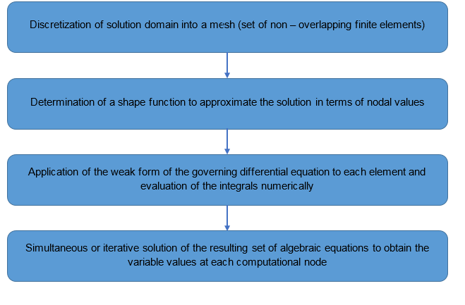
Overall, the finite element approach contains the following steps.

A few of the approaches used to convert the differential equations into their weak integral forms are discussed below.

Weighted Residual Formulation

Substitution of the approximated form into the governing equations results in an error or residual function denoted by

R

and expressed as: (3)

L (\bar{φ}) = R

In order to determine the nodal values

φ_{i}

, the inner product of the residual with a prescribed weighted function

w_{i}

is set to zero (4)

\int_{Ω}^{} R w_{i} d Ω \equiv \int_{Ω}^{} L (\bar{φ}) w_{i} d Ω = 0

The above equation is called the strong form of the weighted residual method. In many cases it is possible to perform integration by parts and obtain the weak form of the equation which contains lower order derivatives than the ones occurring in

L

and has reduced continuity requirement for the weighted function. The weak form is expressed as: (5)

\int_{Γ}^{} A (\bar{φ}) w_{i} d Γ + \int_{Ω}^{} B (\bar{φ}) C (w_{i}) d Ω = 0

where $A$ , $B$ and $C$ are the differential operators with lower order derivatives than $L$ and $Ω$ represents the domain and $Γ$ the boundary of the domain.

Different solution methods are obtained based on the choice of the weight function. Some of these approaches are:

Point Collocation: $w_{i} (x) = δ (x, x_{i})$ where $δ$ is the Dirac-Delta function. This is analogous to the finite difference approach.
Subdomain Collocation: $w_{i} (x) = 1$ for the $i^{t h}$ subdomain (element) and zero elsewhere. This leads to a finite volume formulation.
Galerkin method: $w_{i} (x) = N_{i} (x)$ where $N$ is a shape function assumed over an element.
Petrov Galerkin method: $w_{i} (x) \neq N_{i} (x)$ . This represents a generalization of all methods except the Galerkin method.

Least Squares Formulation

The least square approach is based on minimizing the residual function in a least square sense. A least square function is constructed by taking the inner product of residual function with itself and defined as: (6)

I (\bar{φ}) = L {(\bar{φ})}^{2}

Using variational principles leads to a least square weak form written as: (7)

\int_{Ω}^{} L (w_{i}) L (\bar{φ}) d Ω = 0

Galerkin Least Squares Formulation

Galerkin least square approach is an extension of the Galerkin weighted residual method and the least square approach. It uses stabilizing terms obtained by minimizing the residual of the governing equation. The use of variational principles on the resulting equations results in the following formulation: (8)

L (φ_{i}), w_{i} + S^{G L S} = L (φ_{i}), w_{i} + \sum_{k} L (φ_{i}), τ_{k} L {(w_{i})}_{k} = 0

where

$L (φ_{i}), w_{i}$ represents the Galerkin approximation.
$S^{G L S}$ represents the least squares stabilization.
$〈, 〉$ represents the inner dot product of the comma separated terms.
$τ_{k}$ represents the stabilization parameter.