A Rigid to Rigid contact captures contact forces between two rigid bodies moving
relative to each other in either a 3D frame or a 2D plane.
Define the Connectivity of 3D Rigid to Rigid Contacts
From the Connectivity, the bodies/graphics involved in the contact can be defined.
Checks on graphics for suitability for contacts can also be performed.
If the Contacts panel is not currently displayed, select the desired contact by
clicking on it in the Project Browser or in the modeling window.
The Contacts panel is automatically displayed.
Click the Body I collector and select the first body to
define the contact from the modeling window, or
double-click the collector to open the Model Tree (from
which the desired body can be selected).
In the same manner, click the Body J collector and
select the second body for the contact from the modeling window or Model Tree.
For each of the selected bodies, choose the graphics that are involved in the
contact from the list below the body.
All eligible graphics on a body are automatically selected for contacts.
Individual graphics may be selected/deselected by using the individual check box
located next to each graphic entity in the list.
Alternately, you can click
the Graphic collector to activate it and then simply
select the desired geometry from the modeling window.
Tip:
The All , None , and Reverse options located below the graphic
collector allow you to quickly select the set of graphics you would
like to use for the contact.
Click Material Inside to specify if the
graphic has material inside the volume or outside. When this option
is selected, it means that the selected geometry is solid. In other
words, it is filled with material and its exterior is devoid of
material. Consequently, the surface normals of the geometry point
outward. When the option is not selected, it means the converse is
true: the exterior of the geometry is filled with material and the
interior is devoid of material. In this case, the surface normals of
the geometry point inward. This flag is useful for reversing the
surface normals of a geometry for contact simulations.
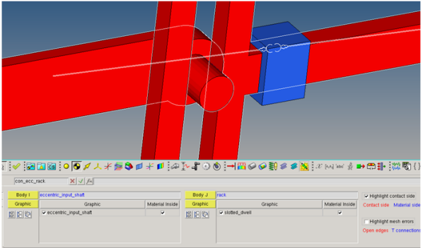
Activate Highlight contact side to visualize
the direction of the contact of the surface mesh. The side of the
surface that would be in contact is indicated by a red color, while
the material side is indicated by a blue color.
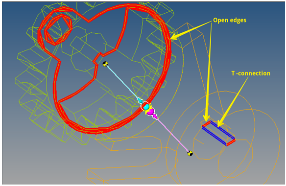
Activate Highlight mesh errors to visualize
any discontinuities in the surface mesh, such as open edges and
T-connections. An open edge is highlighted through a red line, while
a T-connection is highlighted using a blue line. For better
visibility, the visualization of graphic components involved are
changed to a non-shaded mode.
Note: If no mesh errors are found, this
option will be disabled and will display No mesh
errors.
Additional Comments:
In the ADAMS solver mode, if the graphic defined is a File type graphic - it
will require an additional parasolid file.
The individual graphics involved in contact should form a closed volume. In
other words, the graphic mesh should not have any open edges or T-connections.
Use the Highlight mesh errors option to check for open
edges and T-connections. Figure 1.
The normal of the mesh should point in the direction of contact. The side of the
surface mesh, when seen such that the normal direction points towards the viewer
is the contact side. If viewed from the opposite direction, it is referred to as
the material side. Use the Material Inside and
Highlight contact side options in the panel to set
the correct direction of contact. Below is an example of how the Material Inside
and Highlight contact side options work:Figure 2.
With both of the graphics having the Material Inside option activated,
checking the Highlight contact side option will
display the color for both of these graphics in red when viewed from the
outside of the graphics.
In certain cases, if the contact direction is
on the reverse, the Material Inside flag can be flipped.
Define the Connectivity of 2D Rigid to Rigid Contacts
From the Connectivity, the bodies/graphics involved in the 2D contact can be defined.
Checks on graphics for suitability for contacts can also be performed.
Click the Body I collector and select the first body to
define the contact from the modeling window, or
double-click the collector to open the Model Tree (from
which the desired body can be selected).
In the same manner, click the Body J collector and
select the second body for the contact from the modeling window or Model Tree.
For each of the selected bodies, choose the graphics that are involved in the
contact from list below the body.
All eligible graphics on a body are automatically selected for contacts.
Individual graphics may be selected/deselected by using the individual check box
located next to each graphic entity in the list.
Alternately, you can click
the Graphic collector to activate it and then simply
select the desired geometry from the graphics window.
Tip:
The All , None , and Reverse options located below the graphic
collector allow you to quickly select the set of graphics you would
like to use for the contact.
Click Flip Contact Side to to specify the
side of the curve graphic which will come in contact. The side of
the curve as pointed by the arrow indicates its contact side.
Changing this flag will reverse the direction of contact.
Activate Highlight contact side to visualize
the direction of the contact of the curve.
Activate Identity Planarity to check the
planarity of the curves involved in contact. This tool checks
whether the curves are planar and whether the curves are co-planar
considering the first selected graphic in Body I as reference.
Note:
The individual curve graphics involved in 2D contact must use planar curves
only. A planar curve has all of its data points in a single plane.
Currently, MotionView only supports 3D
Cartesian/parametric curves for creating curve graphics that can be used in
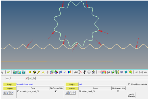
2D contact. Below is an example of how the Highlight contact side option
works: Figure 3.
The example above shows a rack and a pinion
represented with curves and a 2D contact defined between them. The side
of the pinion on which the arrows are pointing (which is outside)
indicate the side the contact is expected. Similarly, the arrows on the
pinion curve have arrows pointing on it from the outside.
In the
case where the contact is expected from the opposite side, the Flip
Contact Side option can be used.
Define the Properties of Rigid to Rigid Contacts
Parameters for normal and friction force calculations are defined in the Properties
tab.
Click the Properties tab.
Use the tabs located at the top of the panel to distinguish between a normal
force or a friction force.
Normal Forces
This tab is used to set the method and related properties to calculate the normal
force during contact. The following four models for defining the normal force are supported:
Impact, Poisson, Volume, and User-Defined.
Click the Normal Force tab.
Select the desired method and define the related properties.
If Impact is chosen:
Enter a value for the stiffness of the boundary surface
interaction.
Stiffness > 0.
Enter a value for the exponent on penetration depth in the
force-penetration depth characteristic of the contact interface.
For a stiffening spring characteristic, it must be greater than 1.0.
For a softening spring characteristic, it must be less than
1.0.
Exponent > 1.
Enter a value for the maximum damping coefficient.
This value should be greater than 0.0.
Enter a value for the penetration depth beyond which full damping is
applied.
If Poisson is chosen:
Enter a value for the penalty parameter to determine the local
stiffness properties between materials.
Larger values lead to reduced penetration between two bodies.
Enter a value for the coefficient of restitution.
This value represents the energy loss between the two contact bodies.
The valid range for this value is between 0.0 and 1.0. A value of 1.0
represents no energy loss and a perfectly elastic contact. A value of
0.0 represents a perfectly plastic contact and all energy is dissipated
during contact.
Enter a value for the normal velocity at which full damping is
applied.
Note: Applicable for the ADAMS solver mode only, click the
Use augmented Lagrangian formulation
option to refine the accuracy of the normal force between the two
bodies.
If Volume Model is chosen:
Enter a value for the bulk modulus of each body.
The bulk modulus of a substance measures the resistance of a substance
to uniform compression. It is defined as the ratio of the infinitesimal
pressure increase to the resulting relative decrease of the volume.
Enter a value for the shear modulus of each body.
The shear modulus or modulus of rigidity is defined as the ratio of
shear stress to the shear strain.
Enter a value for the layer of depth of material for each body.
Enter a value for the exponent of the force deformation
characteristic.
Enter a value for the damping coefficient.
If User-Defined is chosen:
Enter the user subroutine function expression in the in the User expr:
text box.
Activate the Use local file and function name
check box if the use of a local subroutine file is necessary.
Select the subroutine file in the local system by clicking on the
Local File: folder icon.
From the Function Type drop-down menu, select the type of the
subroutine file: DLL/SO,
Python, or MATLAB.
Enter the function name in the Function Name: text box.
MotionView provides CNFSUB as the default,
which is the default function used by MotionSolve and ADAMS.
Refer to the Force_ContactMotionSolve statement for additional details regarding each
method.
Friction Forces
This tab is used to determine the options to include or exclude Coulomb friction in
the calculation of the contact force.
Click the Friction Force tab.
Select the desired method and define the related properties.
If Disabled is chosen, friction is turned off.
If Dynamic Only is chosen, only dynamic friction or
sliding friction is considered in friction calculations. The static regime and
transition to sliding is ignored.
If Static & Dynamic is chosen, all three regimes
are considered in friction calculations: static, transition to sliding friction,
and sliding friction.
The steps needed to define Dynamic Only and Static &
Dynamic friction are the same:
Enter a value in the MU Static field for the static coefficient of
friction, which has to be overcome by a body before it can move.
Note: Not applicable for Dynamic Only.
Enter a value in the MU Dynamic field for the coefficient of friction
that the body experiences while in motion.
Enter a value in the Stiction transition velocity field for the
velocity limit below which the coefficient of friction becomes MU
static.
When the slip velocity is between stiction transition velocity and
friction transition velocity, the coefficient of friction is in
transition between the two.
Note: Not applicable for Dynamic Only.
Enter a value in the Friction transition velocity field for the
velocity above which the coefficient of friction become MU
dynamic.
When the slip velocity is between stiction transition velocity and
friction transition velocity the coefficient of friction is in
transition between the two.
If User-Defined is chosen:
Enter the user subroutine function expression in the User expr: text
box.
Activate the Use local file and function name
check box if the use of a local subroutine file is necessary.
If this option is not specified, MotionSolve will search for a
subroutine following its User Subroutine Loading Rules.
Select the subroutine file in the local system by clicking on the
Local File: folder icon.
From the Function Type drop-down menu, select the type of the
subroutine file: DLL/SO,
Python, or MATLAB.
Enter the function name in the Function Name: text box.
MotionView provides CFFSUB as the default,
which is the default function used by MotionSolve and ADAMS.
Refer to the Force_ContactMotionSolve statement for additional details regarding each
method.
Define the Advanced Options of Rigid to Rigid Contacts
The Advanced tab provides advanced options to control the contact event during
simulation in MotionSolve.
Note: This tab is only available in the MotionSolve
solver mode.
Click the Advanced tab.
Activate one or both of the contact event control options.
Option
Description
Find precise contact event
Activate this option to tell the solver to capture the first event
of contact precisely.
Change simulation max step size
Activate this option to change the maximum step size for the
simulation after contact is detected.
If applicable, enter a value for the max step size scale factor.
Similarly, enter a value for the new max step size.
Note:
Activating Find precise contact event will
automatically introduce a sensor entity in the MotionSolve solver deck which will track the
contact force function.
As the sensor is triggered by a positive contact force, the solver
rejects the last successful step and proceeds from the previous step
size with a changed maximum step size. The changed maximum step size
is calculated as (current max step size) * (Max step size scale
factor).
Activating Change simulation max step size
will enable changing the maximum step size for the future course of
the of the simulation.
Both of the above options provide increased accuracy and robustness
in contact simulations, however they will result in increased
simulation times. It is therefore recommended that these options be
used selectively and only when necessary.
Use the drop-down menu to select where the force will be computed.
Option
Description
Element Center
The contact detection and force calculation in MotionSolve is based on the penetration of mesh
element center. This is the default setting.
Nodes
The contact detection and force calculation in MotionSolve is based on the penetration of mesh
nodes.
 , None
  , and Reverse
  options located below the graphic
collector allow you to quickly select the set of graphics you would
like to use for the contact.
options located below the graphic
collector allow you to quickly select the set of graphics you would
like to use for the contact.