Results at Position - Integration Points
Default option in Abaqus. If the ODB file contains only integration point results, the ODB reader in HyperView extrapolates the results to the element corner nodes in addition to the results for the integration points.
Therefore, you get results for both Position = NODES and Position = Integration Points even if the ODB file only contains integration point results.
1D Elements
| Element Type | Total Number of Integration Points | Result at Integration Point | Maps to Corner (local node) Number | Base Result |
|---|---|---|---|---|
| 2-noded line | 1 3 |
1 1 1 3 |
1 2 1 2 |
Average |
| 3-noded line | 1 2 3 |
1 1 1 2 1 3 |
1 2 1 2 1 2 |
Average |
2D Solid, Axisymmetric, and Membrane Elements
| Element Type | Total Number of Integration Points | Result at Integration Point | Maps to Corner (local node) Number | Base Result |
|---|---|---|---|---|
| 3-noded (TRIA3) | 1 | 1 1 1 |
1 2 3 |
Average |
| 6-noded (TRIA6) | 3 | 1 2 3 |
1 2 3 |
Average |
| 4-noded (QUAD4) | 4 | 1 2 3 4 |
1 2 4 3 |
Average |
| 4-noded (QUAD4) | 1 | 1 1 1 1 |
1 2 3 4 |
Average |
| 8-noded (QUAD8) | 9 | 1 2 3 4 5 6 7 8 9 |
1 5 2 8 - 6 4 7 3 |
Average |
| 8-noded (QUAD8) | 4 | 1 2 3 4 |
1 2 4 3 |
Average |
2D and Axisymmetric Gasket Elements
| Element Type | Total Number of Integration Points | Result at Integration Point | Maps to Corner (local node) Number | Base Result |
|---|---|---|---|---|
| 2-noded link (Rod) | 1 | 1 1 |
1 2 |
Average |
| 4-noded (QUAD4) | 2 | 1 1 2 2 |
1 3 2 4 |
Average |
3D Solid Elements
| Element Type | Total Number of Integration Points | Result at Integration Point | Maps to Corner (local node) Number | Base Result |
|---|---|---|---|---|
| 4-noded (TETRA4) | 1 | 1 1 1 1 |
1 2 4 3 |
Average |
| 6-noded (PENTA6) | 2 | 1 1 1 2 2 2 |
1 2 3 4 5 6 |
Average |
| 8-noded (HEX8) | 8 | 1 2 3 4 5 6 7 8 |
1 2 4 3 5 6 8 7 |
Average |
| 8-noded (HEX8) | 2 | 1 1 1 1 2 2 2 2 |
1 2 3 4 5 6 7 8 |
Average |
| 10-noded (TETRA10) | 4 | 1 2 3 4 |
1 2 3 4 |
Average |
| 15 noded (PENTA15) | 9 | 1 2 3 4 5 6 7 8 9 |
1 2 3 13 14 15 4 5 6 |
Average |
| 20 noded (HEX20) | 27 | 1 2 3 4 5 6 7 8 9 10 11 12 13 14 15 16 17 18 19 20 21 22 23 24 25 26 27 |
1 9 2 12 - 10 4 11 3 17 - 18 - - - 20 - 19 5 13 6 16 - 14 8 15 7 |
Average |
| 20-noded (HEX20) | 8 | 1 2 3 4 5 6 7 8 |
1 2 4 3 5 6 8 7 |
Average |
3D Shell Elements at Each Layer
| Element Type | Total Number of Integration Points | Result at Integration Point | Maps to Corner (local node) Number | Base Result |
|---|---|---|---|---|
| 3-noded (TRIA3) | 1 | 1 1 1 |
1 2 3 |
Average |
| 3-noded (TRIA3) | 3 | 1 2 3 |
1 2 3 |
Average |
| 6-noded (TRIA6) | 3 | 1 2 3 |
1 2 3 |
Average |
| 4-noded (QUAD4) | 4 | 1 2 3 4 |
1 2 4 3 |
Average |
| 4-noded (QUAD4) | 1 | 1 1 1 1 |
1 2 3 4 |
Average |
| 8-noded (QUAD8) | 9 | 1 2 3 4 5 6 7 8 9 |
1 5 2 8 - 6 4 7 3 |
Average |
| 8-noded (QUAD8) | 4 | 1 2 3 4 |
1 2 4 3 |
Average |
3D Gasket Elements
| Element Type | Total Number of Integration Points | Result at Integration Point | Maps to Corner (local node) Number | Base Result |
|---|---|---|---|---|
| 2-noded link (Rod) | 1 | 1 1 |
1 2 |
Average |
| 4-noded (QUAD4) | 2 | 1 1 2 2 |
1 3 2 4 |
Average |
| 6-noded (PENTA6) | 3 | 1 1 2 2 3 3 |
1 4 2 5 3 6 |
Average |
| 8-noded (HEX8) | 4 | 1 1 2 2 3 3 4 4 |
1 5 2 6 4 8 3 7 |
Average |
1st-Order Elements
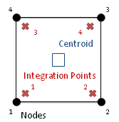
Figure 1.
| Key | S-Stress Components (s) | Key | S-Stress Components IP (s) |
|---|---|---|---|
 |
Integration point results are extrapolated to the element corners when Display corner data is selected. Abaqus proprietary shape functions and APIs are used. |
|
Integration point results are at the nearest element corners when Display corner data is selected. Results are not extrapolated. |
 |
Average of nodes 1, 2, 3, and 4, when Display corner data is deselected. |
|
Average of integration points 1, 2, 3, and 4 when Display corner data is deselected. |
2nd-Order Elements
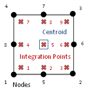
Figure 2.
| Key | Key | ||
|---|---|---|---|
|
|
Integration point results are extrapolated to element corners using Abaqus proprietary API and shape functions. |
|
Integration point (IP) results are at the nearest element corners when Display corner data is selected. Results are not extrapolated. Center IP result is ignored. |
|
|
Average of all extrapolated nodal results when Display corner data is off. |
|
Average of all integration points when Display corner data is deselected. |
Results at Position - Nodes
The data type names without the "IP" suffix contain the nodal tensor (ELEMENTAL_NODAL) results as the corner result.
The Abaqus ODB reader reads these values directly from the ODB file (or extrapolates them from the integration point results) and assigns them to the corner of each element. In HyperView, the Display corner data option on the Contour panel has to be selected to plot the contour with corner results.
Von Mises Stress Output for Random Response Analysis
HyperView supports RMS von Mises Stress and von Mises Stress results for Random response analysis.
The output variable “MISES-Mises stress based on segalman(s)” is the von Mises Stress and “RMISES-RMS of Mises stress based on Segalman(s)” is the RMS von Mises Stress output. To calculate the MISES and RMISES output stress value at element level is needed. So in random response analysis the stress output must be requested in the preceding frequency step. These data’s stored in the odb file is extracted in the reader and the actual computation is done based on work by Segalman, et al. (1998).
 is the Mises stress calculated based on Segalman, et
al. (1998),
is the Mises stress calculated based on Segalman, et
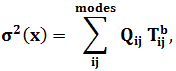
al. (1998),  , is the PSD matrix containing all the frequency
related term and
, is the PSD matrix containing all the frequency
related term and  , is the stress output for a particular node b.
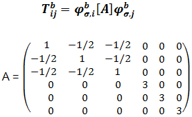
 and
and  represent the stress components for
  and
and  mode at a given node b and A is a constant matrix. The
RMS von mises at a node b is calculated using the following equation:
mode at a given node b and A is a constant matrix. The
RMS von mises at a node b is calculated using the following equation:
Limitation: The calculation time can be high for big models. In this case, results can be extracted in batch mode using HVTrans.