Create Iso Surfaces for Elemental Results
-
From the View Controls toolbar, click
 .
.
-
From the Iso panel, select the data type that should be used to calculate the
iso values from the Result type drop-down menu.
The available result types change depending on the result file that is loaded.Each result type is followed by a letter that indicates the category to which it belongs. (t) indicates a tensor-type result, such as stress or strain tensors. (v) indicates a vector-type result, such as displacement, velocity, and acceleration. (s) indicates a scalar-type result. (c) indicates complex results.Tip: Click the expansion button
 to open the Choose From List
dialog, where you can filter result types for faster selection.
to open the Choose From List
dialog, where you can filter result types for faster selection. -
If the element has layers defined, select the relevant option for Entity with
layers.
The settings are applied to all layers defined in the model. If an element has no layer definition, as with solids, the iso surfaces are displayed regardless of layer selection.
Option Description Max Displays the maximum value among the layers for each entity. Min Displays the minimum value among the layers for each entity. Extreme Displays the maximum absolute values among the layers for each entity. Sum Displays the (scalar) sum of all values among the layers for each entity. Average Displays the (scalar) average value among the layers which contain data for each entity. Layers that do not have values (N/A result) will not contribute to the averages (see the example below):
Layer 1 - 10.0
Layer 2 - 26.0
Layer 3 - 30.0
Average is (10+26+30)/3 = 66/3 = 22.0
However if:
Layer 1 - 10.0
Layer 2 - 26.0
Layer 3 - N/A
Average is (10+26)/2 = 36/2 = 18.0
Range Displays the difference between the maximum and minimum values among the layers for each entity. Count Displays a count of the layers for the given data type. By default, the total number of layers/plies are given for each node/element. When used with a Layer Filter or Value Filter, the Count aggregation mode will have slightly different behavior (based on the filter criteria). MaxLayer Plots an iso-surface based on the available layer index that contributes to the maximum value for each entity. MinLayer Plots an iso-surface based on the available layer index that contributes to the minimum value for each entity. ExtremeLayer Plots an iso-surface based on the available layer index that contributes to the extreme (absolute maximum) value for each entity. Solver specific layer options Solver dependent label(s). For example, Z1 and Z2 would indicate the lower and upper layers of shells in a Nastran model. Tip: Use the Layer Filter to reduce the layer list
available for aggregation for the data types which have layers (for example,
plies in composite stress/stains or any vector result with layers).Note: Only in the case of results based at the elemental centroid, would one layer per element be displayed. For corner bound or nodal bound results (in the case of averaging), different layers may contribute to the max/min/extreme value at each corner/node of the same element.
to reduce the layer list
available for aggregation for the data types which have layers (for example,
plies in composite stress/stains or any vector result with layers).Note: Only in the case of results based at the elemental centroid, would one layer per element be displayed. For corner bound or nodal bound results (in the case of averaging), different layers may contribute to the max/min/extreme value at each corner/node of the same element.When plotting an iso-surface for MaxLayer, MinLayer, or ExtremeLayer, a layer index which may be specific to the file is used. This index does not provide you with any useful information, therefore the iso-surface plot by itself will not be effective without an accompanying contour plot. In addition, the Current Value or the Slider for changing the iso-surface values is not recommended when using MaxLayer/MinLayer/ExtremeLayer.
See the Derived Load Steps topic to view a table which explains the behavior of layer aggregation (Min/Max/Range) in combination with the Min/Max/Range Envelope loadstep types.
-
Before creating an iso plot, you may pick one or more components from the
model.
- Click the Components input collector and use the extended entity selection menu.
- Pick entities directly from the model in the modeling window.
Note: If no selection is made, the iso plot will be applied to displayed components by default.Component selection restricts the iso surface to the selected parts only, while displaying the rest of the geometry which needs to be displayed in full. In most of the CFD applications, the fluid elements need to be iso surfaced, with the structural parts displayed as a whole. The figure below shows a pump impeller geometry, with the iso surface on the fluid elements based on pressure data. The contour shown is velocity of the fluid as it is displaced by the impeller blade.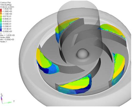
Figure 1.When performing ALE simulations in Radioss, or other solvers, of fuel tank sloshing or ditching of an airplane, the iso surface of density on selected components (the mesh representing the fluid) helps visualize the interaction of the fluid with the structure. The image below shows a ditching simulation of an airplane in water. The airplane block is investigated while the density iso surface is applied only on the fluid to show the water displacement due to ditching.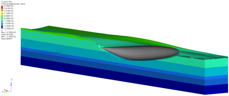
Figure 2. -
Select an averaging method from the drop-down menu.
Averaging Method Description None When elemental centroidal results are used, None is not available in the Iso panel since node based results are required to generate an iso value. So, if you apply elemental centroidal results, you need to select one of the averaging methods. If nodal results are used, no selection of averaging methods is possible.
Simple Tensor and vector components are extracted and the invariants are computed prior to averaging. Note: This is the default setting.Maximum Extracts the maximum values from the surrounding elements attached to a node. The tensor and vector components are extracted and the invariants are computed for each element (or corner) prior to averaging to a node. For results components, the corresponding components from each element corner (or centroid) are extracted and then the maximum value is assigned to the shared node. For invariants, the corresponding invariants are calculated from each tensor at the element corners and then the maximum value is assigned to the node. For example, as shown in the Nodal Averaging of Elemental Results topic, there are four tensors, [A2], [B1], [C3], and [D4] at four corners at Node 400.
The maximum average of the xx component at Node 400 is:
Minimum Extracts the minimum values from the surrounding elements attached to a node. The tensor and vector components are extracted and the invariants are computed for each element (or corner) prior to averaging to a node. For results components, the corresponding components from each element corner (or centroid) are extracted and then the minimum value is assigned to the shared node. For invariants, the corresponding invariants are calculated from each tensor at the element corners and then the minimum value is assigned to the node. For example, as shown in Nodal Averaging of Elemental Results, there are four tensors, [A2], [B1], [C3], and [D4] at four corners at Node 400.
The minimum average of the xx component at Node 400 is:
Advanced Tensor (or vector) results are transformed into a consistent system and then each component is averaged separately to obtain an average tensor (or vector). The invariants are calculated from this average tensor. Difference The difference between the maximum and minimum corner results at a node. Max of corner Extracts the maximum value from all the corners of an element and the value is shown at the centroid of the element. The tensor and vector components are extracted and the invariants are computed for each corner prior to assigning to the element centroid. For result components, the corresponding components from each corner is extracted and then the maximum value is assigned to the element centroid. For invariants, the corresponding invariants are calculated from each tensor at the element corners and then the maximum value is assigned at the centroid. For example, as shown in Nodal Averaging of Elemental Results, there are four tensors at each corner of the element A: [A1], [A2], [A3], and [A4].
The max of corner aggregation of the xx component at the Element A centroid is:
This averaging option is only available when the Use corner data option is checked. The Variation option is automatically disabled for this averaging method.
Min of corner Extracts the minimum value from all the corners of an element and the value is shown at the centroid of the element. The tensor and vector components are extracted and the invariants are computed for each corner prior to assigning to the element centroid. For result components, the corresponding components from each corner is extracted and then the minimum value is assigned to the element centroid. For invariants, the corresponding invariants are calculated from each tensor at the element corners and then the minimum value is assigned at the centroid. For example, as shown in Nodal Averaging of Elemental Results, there are four tensors at each corner of the element A: [A1], [A2], [A3], and [A4].
The min of corner aggregation of the xx component at the Element A centroid is:
This averaging option is only available when the Use corner data option is checked. The Variation option is automatically disabled for this averaging method.
Extreme of corner Extracts the extreme value from all the corners of an element and the value is shown at the centroid of the element. The tensor and vector components are extracted and the invariants are computed for each corner prior to assigning to the element centroid. For result components, the corresponding components from each corner is extracted and then the extreme value is assigned to the element centroid. For invariants, the corresponding invariants are calculated from each tensor at the element corners and then the extreme value is assigned at the centroid. For example, as shown in Nodal Averaging of Elemental Results, there are four tensors at each corner of the element A: [A1], [A2], [A3], and [A4].
The extreme of corner aggregation of the xx component at Element A centroid is:
This averaging option is only available when the Use corner data option is checked. The Variation option is automatically disabled for this averaging method.
-
Click the Averaging Options button and select from the
options available in the Averaging Options dialog.
The averaging options allow you to limit the averaging of results to only a group of elements that are considered to be bound by same feature angle or face.
Typically averaging is performed for all connected elements in a part without any regard for adjacent elements that are modeled around sharp edges or T-connections
Note: Feature angle averaging is only applicable when the Simple or Advanced averaging methods are used, and no Variation is selected. As the nodes shared by elements that do not meet the feature angle criteria can have different values on either side of the feature angle, the output is always presented as corner bound values on each element.Option Description Average across component boundary Enables the nodal averaging across the component boundary. The contribution for a shared node will come from every component associated with that node, while all of the other averaging principles remain. Feature angle averaging Activate this option to specify the threshold value for elements to be considered as part of the same feature by specifying a Feature angle value. All of the adjacent elements whose normals are less than or equal to the threshold value are averaged. The output of this contour is always corner based data (no centroid values). A feature angle average calculation example is shown below: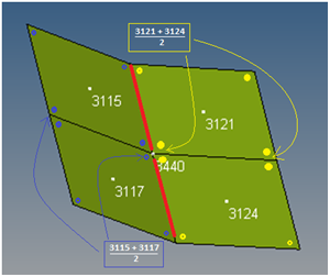 Result at common node 3440:
- E 3115, average of corner nodes for element 3115 and 3117
- E 3121, average of corner nodes for element 3121 and 3124
- E 3117, average of corner nodes for element 3115 and 3117
- E 3124, average of corner nodes for element 3121 and 3124
Feature angle Allows you to specify the value to be used in the Feature angle averaging calculations. The default is 30 degrees. All of the elements whose normals are less or equal to the specified threshold value are averaged. The value can range from 0 to 180 degrees. For element feature angle calculation, the current model position is used. Only shell elements feature angles are considered, therefore all solid and beam elements will be included in the averaging calculation (see the example below):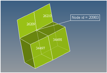
The result at common node 20983 = the average of corner nodes for all four elements.
Ignore flipped normals This option is checked by default (for feature based averaging) to allow for any modeling discrepancies to be disregarded. Consider the picture and description below which shows two adjacent elements whose normals are flipped as a consequence of a model setup discrepancy: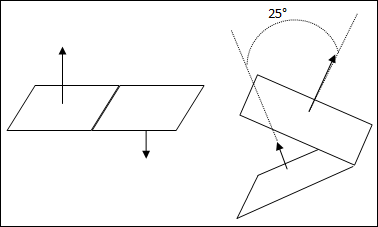
In the example above, the feature angle threshold for averaging is set at 30 degrees. The image on the left side has an angle between adjacent element normals close to 180 degrees and therefore does not meet the criteria of the 30 degree threshold. The image on the right has the angle between normals less than 30 degrees, and the threshold criteria for feature angle is satisfied. However, this could be a modeling discrepancy that should be accounted for, perhaps allowing the averaging of values for elements on the left image, but not allowing averaging of elements on the right image. This can be accomplished by activating the Ignore flipped normals option.
If strict adherence to the angle between adjacent element normals is to be enforced, then uncheck this option.
Note: The Legend will automatically update and reflect that feature angle averaging is activated.