AutoBush
The AutoBush is a bushing model that is designed to easily simulate bushings used in ground vehicles. The AutoBush entity reads bushing stiffness (force-displacement) and damping (force-velocity) data from a file written in the TeimOrbit format.
- Forces-deflection properties are stored in one ASCII format file, called the property file.
- Multiple bushings may reference the same property file.
- The property file format is compatible with other MBD codes, such as SIMPACK and ADAMS.
- Bushing Coupling is supported as a user selected choice.
The AutoBush entity uses a Force_field XML statement in the MotionSolve deck, along with a subroutine to calculate the bushing forces and moments. The bushing property file is read by MotionSolve at the beginning of the simulation. MotionSolve uses Akima’s method to interpolate the force-deflection curves stored in the property file. For deflections outside the range in the property file, MotionSolve linearly extrapolates forces and/or moments.
Bushing Graphic
A bushing graphic appears when an AutoBush entity is added using the interface. The graphic includes a cylinder, and two large X-Y local coordinate frame indicators.
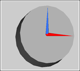
Figure 1. AutoBush Bushing Graphic
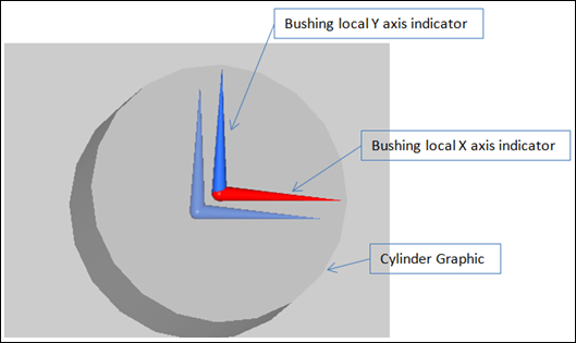
Figure 2. AutoBush Bushing Graphic-Cylinder Graphic (shown as transparent)
Coupling
- Method
- Description
- Rectangular
- The displacement on each axis of the bushing is computed independently.
- Cylindrical
- Couple the X and Y displacements (translational and rotational). The radial
deflection (r) is given by:
r = sqrt( x^2 + y^2 )
Fx = x/r*Gx( sign(x)*r )
Fy = y/r*Gy( sign(y)*r )
- Spherical
- Couple the X, Y, and Z direction displacements (translational and rotational). The
radial deflection (r) is given by:
r = sqrt( x^2 + y^2 + z^2 )
Fx = x/r*Gx( sign(x)*r )
Fy = y/z*Gy( sign(y)*r )
Fz = z/r*Gz( sign(z)*r )
Connecting an AutoBush
Connections define the two connecting bodies, the point where the forces act, and the marker that defines the bushing orientation. Bodies, Markers, and Points can be selected either graphically or through the Project Browser.
TeimOrbit Bushing File
- HEADER
- The header block describes the format of the file, if it was written from a pre-processor.
- UNITS
- The units block describes the data in the file.
- DAMPING
- The damping in the bushing. Linear damping is supported in this bushing model and is shown in the file below.
- FX_CURVE, FYCURVE, etc.
- The Displacement vs Force data for the degree of freedom identified in the block header. Enter the data in ascending order.
$-------------------------------------------------------------------HEADER
[HEADER]
 FILE_TYPE     =  'bus'
 FILE_VERSION  =  4.0
 FILE_FORMAT   =  'ASCII'
$------------------------------------------------------------------UNITS
[UNITS]
 LENGTH =  'mm'
 ANGLE  =  'degrees'
 FORCE  =  'newton'
 MASS   =  'kg'
 TIME   =  'second'
$-----------------------------------------------------------------DAMPING
[DAMPING]
 FX_DAMPING  =  0.5
 FY_DAMPING  =  0.5
 FZ_DAMPING  =  0.5
 TX_DAMPING  =  0.5
 TY_DAMPING  =  0.5
 TZ_DAMPING  =  0.5
$----------------------------------------------------------------FX_CURVE
[FX_CURVE]
{  x         fx}
-10.0  -45000.0
 -8.0  -36000.0
 -6.0  -27000.0
 -4.0  -18000.0
 -2.0   -9000.0
  0.0       0.0
  2.0    9000.0
  4.0   18000.0
  6.0   27000.0
  8.0   36000.0
 10.0   45000.0
$----------------------------------------------------------------FY_CURVE
[FY_CURVE]
{  y          fy}
-10.0  -45000.0
 -8.0  -36000.0
 -6.0  -27000.0
 -4.0  -18000.0
 -2.0   -9000.0
  0.0       0.0
  2.0    9000.0
  4.0   18000.0
  6.0   27000.0
  8.0   36000.0
 10.0   45000.0
$----------------------------------------------------------------FZ_CURVE
[FZ_CURVE]
{  z         fz}
-10.0  -45000.0
 -8.0  -36000.0
 -6.0  -27000.0
 -4.0  -18000.0
 -2.0   -9000.0
  0.0       0.0
  2.0    9000.0
  4.0   18000.0
  6.0   27000.0
  8.0   36000.0
 10.0   45000.0
$----------------------------------------------------------------TX_CURVE
[TX_CURVE]
{  ax          tx}
-45.0  -2025000.0
-36.0  -1620000.0
-27.0  -1215000.0
-18.0   -810000.0
 -9.0   -405000.0
  0.0         0.0
  9.0    405000.0
 18.0    810000.0
 27.0   1215000.0
 36.0   1620000.0
 45.0   2025000.0
$----------------------------------------------------------------TY_CURVE
[TY_CURVE]
{  ay          ty}
-45.0  -2025000.0
-36.0  -1620000.0
-27.0  -1215000.0
-18.0   -810000.0
 -9.0   -405000.0
  0.0         0.0
  9.0    405000.0
 18.0    810000.0
 27.0   1215000.0
 36.0   1620000.0
 45.0   2025000.0
$----------------------------------------------------------------TZ_CURVE
[TZ_CURVE]
{  az          tz}
-45.0  -2025000.0
-36.0  -1620000.0
-27.0  -1215000.0
-18.0   -810000.0
 -9.0   -405000.0
  0.0         0.0
  9.0    405000.0
 18.0    810000.0
 27.0   1215000.0
 36.0   1620000.0
 45.0   2025000.0