Cars and Trucks
Altair Driver is a simple driver model. This is used in all MotionView and MotionSolve vehicle events. The controller can predict the future road path based on the current vehicle state, has knowledge of the vehicle dynamics, and has access to user-defined driver parameters.
Input driver parameters specify the control priorities of the driver. Vehicle parameters are used to estimate the vehicle’s future states, based on a simple linear bicycle model. The following paragraphs describe vehicle and driver parameters and their effects on the trajectory planning.
- Usage
-
Altair Driver is implemented as a Control State Equation (CSE). The outputs from the CSE (Throttle, Brake, Steer, Gear and Clutch) are used in the Powertrain, Brake and Steering system. When a vehicle event is selected from the Analysis Wizard in MotionView, the driver is automatically added to the multi-body model as are the required entities (arrays, solver variables, and so on).
- Theory
-
The well-known bicycle model is used as a first approximation to represent a multi-wheeled road vehicle.
There are two control models for the Steering control.- Kinematic bicycle model
- Dynamic bicycle model
- Kinematic Bicycle Model
-
In Kinematic bicycle model, the equations of motion are based purely on geometric relationships governing the system. The major assumption used in the development of the kinematic model is that the velocity vectors at points A and B are in the direction of the orientation of the front and rear wheels respectively. This is equivalent to assuming that the "slip angles" at both wheels are zero. This is a reasonable assumption for low speed motion of the vehicle (for speeds less than 5 m/s). This model does not consider the vehicle’s dynamics such as slipping and skidding.
The kinematic equations of the bicycle model are written in terms of coordinates of the vehicle which gives our three degrees of freedom non-linear model
 .
.The equations on motion written as a set of three differential equations where the state vector is:

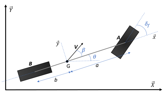
Figure 1.The quantities are:
- Vehicle Yaw Angle

- Lateral Displacement of the vehicle

- Longitudinal Displacement of the vehicle
Equations of motion can be written as:
where,
 - Velocity of the vehicle
 - Rear axle to CG distance
 - Slip angle at the center of gravity
 - Dynamic Bicycle Model
-
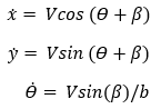
At higher vehicle speeds, the assumption that the velocity at each wheel is in the direction of the wheel can no longer be made. In this case, instead of a kinematic model, a dynamic model for lateral vehicle motion is needed.
The force equations of the bicycle model are written in terms of coordinates of the vehicle which gives our five degrees of freedom non-linear model
.
Figure 2.The equations on motion are written as a set of five differential equations where the state of vector is:
 The quantities are:
- Lateral Velocity of the vehicle

- Yaw rate of the vehicle
- Vehicle Yaw Angle
- Lateral Displacement of the vehicle
- Longitudinal Displacement of the vehicle

- Road wheel steering angle (directly proportional to the steering wheel angle by a rack-pinion reduction ratio)
Using Newton's second law of motion, the equations can be written as:
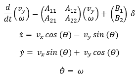
where,
 where,
- Velocity of the vehicle

- Cornering stiffness of (single) front tire

- Cornering stiffness of (single) rear tire

- Mass of the vehicle

- Yaw inertia of the vehicle

- Steering ratio of the vehicle

- Number of front tires

- Number of rear tires

- Front axle to CG distance
- Rear axle to CG distance
In case of multi-axle vehicles (>2),
 and
and
 are calculated according to the vehicle’s axle
configuration and are used as a and b in the above equations.
are calculated according to the vehicle’s axle
configuration and are used as a and b in the above equations.Once the equations of motion have been written, the problem becomes that of classical control theory. The goal is to calculate the steering wheel angle that would cause the vehicle to follow a prescribed path as closely as possible.
This can be achieved in many ways. One strategy could be to use optimal control theory and minimize a cost function measuring a series of weighted factors (including lateral position error, hand-wheel steering angle, and heading error) evaluated at different time steps.
With Altair Driver, MotionSolve computes the error between the predicted path and the desired path at some point in the future. The controller has full knowledge of the vehicle dynamics equations as described above and can compute the predicted position based on those equations at some future time.
To compute the predicted path, the equations of motion are integrated for look-ahead times using the Runge-Kutta integration scheme. The path is obtained by spline interpolation using the spline utility in MotionSolve.
The difference between the predicted path and desired path at look-ahead is the error.
Thus:

The algorithm attempts to estimate the error by evaluating its sensitivity to the steering wheel angle. Convergence is achieved when the error is less than a certain tolerance.
The final steering wheel angle is calculated by the iterative method described below:- Two appropriate steering wheel angle values are chosen and called
 and
and  .
. -
is chosen as the current steering angle and is the current steering angle plus 1 degree.
- The corresponding errors
 and
and
 are calculated and a steering wheel angle,
  , is chosen by linear interpolation using the following
formula:
, is chosen by linear interpolation using the following
formula: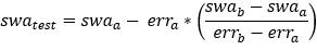
- If the error corresponding to the steering wheel angle is
less than a certain tolerance, then it is used as the steering wheel angle at the
next time step.
- If the error corresponding to the steering wheel angle is
more than the tolerance, then the or which resulted in more error is replaced by and Step 2 is performed again.
- Finally, if the steering wheel angle does not converge after 20 iterations, an error is thrown and the simulation is stopped, signaling the fact that the vehicle cannot perform the path following maneuver.
The final steering wheel angle is essentially used as an increment to the current steering wheel angle as shown below. When computing the new steering wheel angle value (at time t+1), the previous value of the steering wheel angle (at time t) is updated by the quantity:
 Where,
- The step size (the difference between the last successful integration time and the current time).

- The feedback frequency which captures the driver reaction times (should be less than the step frequency).
- Limitations
-
The Kinematic model is valid only for low speed motion of the vehicle. At higher velocities, considerable slip angles are generated on the wheels which is not accounted in this model.
For the Dynamic bicycle model, we have assumed that the lateral tire force is proportional to slip angle. This relationship is valid for smaller slip angles. Since the controller uses this simplified linear representation of the vehicle, its applicability is limited to the linear range.
- User Inputs
-
You can enter vehicle parameters and driver parameters in the Altair Driver panel. The vehicle parameter array contains quantities that are used in the definition of the bicycle model.
These include:- Rear WC to CG long distance ()
- Front WC to CG long distance ()
- Vehicle Mass ()
- Vehicle yaw inertia ()
- Front tire cornering stiffness ()
- Rear tire cornering stiffness ()
You can also click the Calculate button on the Altair Driver panel to update these (except
and ) as well as brake and drivetrain parameters from the
vehicle.In addition to these, the mathematical model also uses Steering ratio (ratio between steering wheel angle input and the road wheel steer angle) which is calculated by the driver before running transient maneuver.
Other driver parameters that influence the driver behavior include:- Look ahead value [s]
- Feed frequency value () [-]
- Maximum steering wheel angle [deg]
- Minimum steering wheel angle [deg]
- Path reference maker (usually a road reference marker present in the tire system)
The maximum steering wheel angle is ultimately used as cut-off value for the computed steering wheel angle.
- Rear WC to CG long distance (