Leaning Two and Three Wheeler Vehicles
- Lean Angle Profile Control
-
The user input for this control algorithm is the target lean angle profile. The steer angle/steer torque is calculated in order to reach the demand lean angle. The calculation is done using PID algorithm.
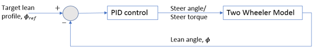
The relation between steer angle/steer torque and the target lean angle can be expressed as:
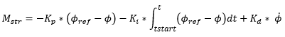
where
 is the target lean angle,
  is the current lean angle and
  is steer angle or steer torque depending on user
selection of driver output.
is steer angle or steer torque depending on user
selection of driver output. ,
,  ,
,  are the PID constants. For steer angle as the control
signal, the constants are parametrized with respect to the inverse of longitudinal
velocity squared.
are the PID constants. For steer angle as the control
signal, the constants are parametrized with respect to the inverse of longitudinal
velocity squared.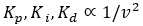
- Path Following Control
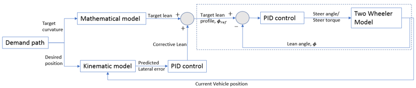
- The user input for this control algorithm is the path defined with respect to path
reference marker on which the two-wheeler needs to be driven. The steer angle/steer
torque is calculated using a combination of feedforward and feedback algorithm.
The demand lean angle is calculated at each time step to follow the upcoming demand path trajectory as well as remove any lateral error with respect to the demand path. This demand lean angle is provided to the lean control algorithm (discussed in the Lean Angle Profile Control section above) to calculate steer angle/steer torque.
-
- Steer Control Algorithm
-
The feedforward algorithm is based on the curvature of the demand path and the predicted lateral error of the vehicle after look ahead time.
The relationship between lean angle and the curvature of the demand path can be established by balancing the lateral acceleration and gravity acting at the center of gravity.
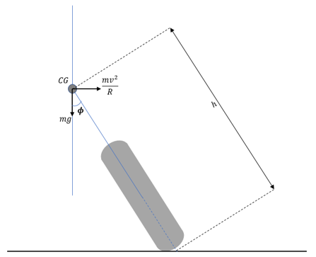
Solving for equilibrium, we get:
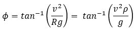
where,
 is longitudinal velocity of the vehicle and
  is the curvature of the path.
Curvature of the path is estimated as given in the Curvature Estimation section.
Accounting for gyroscopic forces at the center of the wheel, the relationship is given as below.
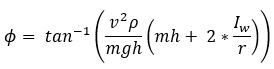
 – mass of the vehicle – longitudinal velocity of the vehicle
 – Inertia of the wheel
 – Radius of the wheel
 – Height of center of gravity of the vehicle – Curvature of the path
 - Curvature Estimation
- The demand curvature is estimated using three points on the demand path. These
three points are spaced using the parameter look ahead time
(lat).
The points P1, P2 and P3 on the path are calculated as:

Where
 is the current position of the vehicle along the
reference path and
is the current position of the vehicle along the
reference path and  is look ahead time.
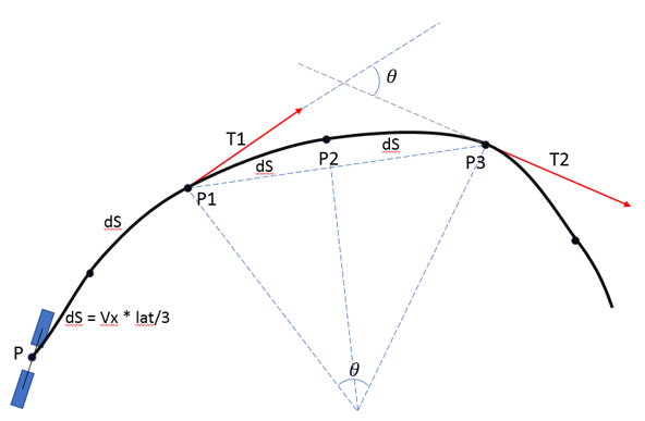
To estimate the curvature using these three points, the tangent vector at these three points (T1, T2 and T3) are found using the path interpolated using quintic spline utility from MotionSolve.
The angle between the tangents is found as:
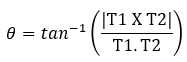
The curvature is estimated as:

- Lateral Error Prediction
- Lateral error is calculated using desired and predicted position of the
vehicle after look ahead time.
To predict the vehicle position after look ahead time, kinematic bicycle model equations are used.
For details on kinematic model, please see the Kinematic bicycle model section.
To compute the predicted path, the equations of motion are integrated for look-ahead times. The path is obtained by spline interpolation using the spline utility in MotionSolve.
The difference between the predicted path and desired path at look ahead time is the error.

- Handling Demand Path with Discontinuous Curvature
-
Some examples for paths with discontinuous curvatures are:
- 90 degrees left/right turn
- Straight line merging to a curved path with constant radii
- Single lane change / Double lane change
The demand lean for the path following control should be continuous in nature to ensure smooth behavior of the control algorithm. As observed in real life as well, smooth cornering is observed when two-wheeler is leaned gradually from one state to another in a continuous fashion.
Since demand lean is directly proportional to the curvature of the path, it is required that the path followed by the driver has continuous curvature, in other words, the second derivative of the path curve should be continuous in nature at each point on the path.
To fulfil this requirement for every path provided by the user, the path curve is sampled at a fixed distance covering the whole path. A quintic (Fifth order) curve is fitted with the sampled points using MotionSolve QUINTIC curve utility. Due to the nature of the curve, the resultant curve has continuous curvature along the whole path. This resultant smooth path is provided to Altair Driver as the new Demand path.
The sampling distance for the path can be set in ADF. The default value for the parameter is 10 m.