Computation Settings
- 3D ray-tracing
- rural ray-tracing model
- one slope model
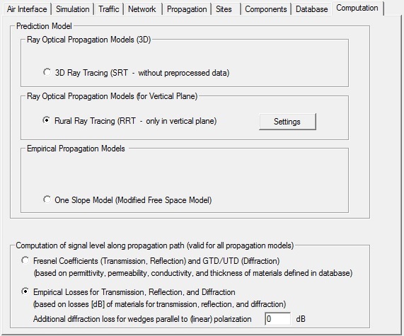
Figure 1. The Computation dialog.
- Prediction Model
- Different models using different computation approaches can be selected. The settings of the models can be changed by using the Settings button.
- Computation of signal level along propagation path (valid for all propagation models)
- The deterministic mode uses Fresnel Equations for the determination of the
reflection and transmission loss and the GTD / UTD for the determination of the
diffraction loss. This model has a slightly longer computation time and uses
four physical material parameters (thickness, permittivity, permeability and
conductivity). When using GTD / UTD and Fresnel coefficients arbitrary linear
polarizations (between +90° and –90°) can be considered for the transmitters.
The empirical mode uses five empirical material parameters (minimum loss of incident ray, maximum loss of incident ray, loss of diffracted ray, reflection loss, transmission loss). For correction purposes or for the adaptation to measurements, an offset to those material parameters can be specified. Herewith the empirical model has the advantage that the needed material properties are easier to obtain than the physical parameters required for the deterministic model. Also the parameters of the empirical model can be calibrated with measurements more easily. It is therefore easier to achieve a high accuracy with the empirical model.
The diffraction loss depends besides the angles of the given propagation path also on the relationship between the wedge direction and the polarization direction. According to physics and verified by measurements there is an additional loss of about 5 dB if both directions are parallel (for example, diffraction on vertical wedge for vertically polarized signal). While this effect is automatically considered if using the GTD / UTD model, an offset is available for the empirical diffraction model. This additional loss is added to the diffraction loss in case the wedge direction and the polarization direction are parallel. In case the wedge direction and the polarization direction are orthogonal no additional loss is considered. In between there is a linear scaling of this additional loss.Note: The computation mode for the signal level along the propagation path applies for all propagation models.