Rural Dominant Path Model
The Dominant Path Model uses a full 3D approach for the path searching, which leads to realistic and accurate results.
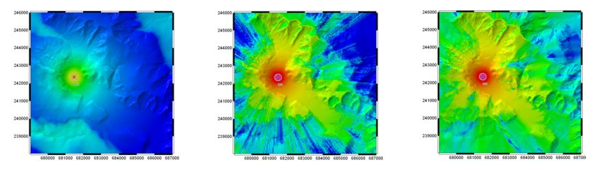
Figure 1. Comparison of results between the Hata-Okumura (on the left), knife-edge diffraction (middle) and dominant path models (to the right).
The simple approach of the Hata-Okumura Model is clearly visible in the left image. Topography between transmitter and receiver is not considered. In contrast to this case, the Knife-Edge Diffraction Model considers topography, but the effects are too dominant. The shadows behind the hills are too hard, because always the direct ray is considered. This leads to too pessimistic results. The Dominant Path Model uses a full 3D approach for the path searching, which leads to realistic and accurate results.
Advantages of the Dominant Path Model
- The most important propagation path is computed by using a full 3D approach
- Short computation times
- Accuracy exceeds the accuracy of empirical models
Algorithm of the Dominant Path Model
The DPM determines the dominant path between transmitter and each receiver pixel. The computation of the path loss is based on the following equation:
- Distance from transmitter to receiver (l)
- Path loss exponent (p)
- Wave length (lambda)
- Individual interaction losses due to diffractions (f)
- Gain of transmitting antenna (gt)
As described above, l is length of the path between transmitter and current receiver location. p is the path loss exponent. The value of p depends on the current propagation situation. In areas with vegetation (which is not modeled in the project) p = 2.4 is suggested, whereas in open areas p = 2.0 is reasonable. In addition p depends on the breakpoint distance. After the breakpoint, increased path loss exponents are common due to distortions of the propagating wave. The function f yields the loss (in dB) which is caused by diffractions. The diffraction losses are accumulated along one propagation path. The directional gain of the antenna (in direction of the propagation path) is also considered.
Configuration of the Dominant Path Model
The following screenshot shows the configuration dialog of the DPM.
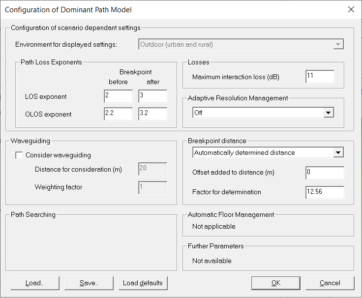
Figure 2. The Configuration of Dominant Path Model dialog.
- Path Loss Exponents
- The path loss exponents influence the propagation result computed by the DPM
significantly. The path loss exponents describe the attenuation with
distance. A higher path loss exponent leads to a higher attenuation in same
distance. The following figure shows a comparison of three predictions with
different path loss values for the LOS area.
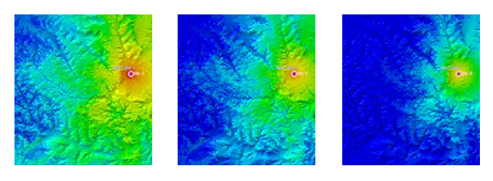
Figure 3. Comparison of path loss predictions with different path loss values. LOS exponent 2.0 (on the left), LOS exponent 2.3 (middle) and LOS exponent 2.6 (to the right). - Losses
- Each change in the direction of propagation due to an interaction (diffraction, transmission/penetration) along a propagation path causes an additional attenuation. The maximum attenuation can be defined. The effective interaction loss depends on the angle of the diffraction. It is recommended to leave the default value.
- Adaptive Resolution Management
- For acceleration purposes, the DPM offers an adaptive resolution. In close streets a fine resolution is used for the prediction and on large places or open areas DPM switches automatically to a coarse resolution. The prediction time and the memory demand are positively influenced by the adaptive resolution but the accuracy is limited - especially if the highest level for the adaptive resolution is selected by the user.
Additional Features
- Consideration of clutter in rural/suburban environment: Clutter databases describe the land usage of scenarios and can be considered by the DPM.
- Auto calibration of model parameters.
Auto Calibration
The model can be calibrated automatically.