Knife Edge Model
This model takes the effect of the actual environment into account by using 3D vector building data (plus terrain profile).
Deterministic models utilize physical phenomena to describe the propagation of radio waves. Herewith the effect of the actual environment is taken into account by using 3D vector building data (plus terrain profile). Generally deterministic propagation models are based on ray-optical techniques. A radio ray is assumed to propagate along a straight line influenced only by the present obstacles which lead to reflection, diffraction and the penetration of these objects. However, for large distances between transmitter and receiver, especially for satellite transmitters, the computational demand is still challenging. For some scenarios there is no 3D vector data of the environment available but clutter height information describing the building heights in pixel format. In both cases the knife edge diffraction model provides an efficient approach for the coverage prediction based on either vector or pixel data (including building and topographical data).
Parameters
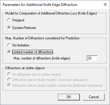
Figure 1. The Parameters for Additional Knife Edge Diffraction dialog.
- Model for computation of additional diffraction loss
- Model for determination of knife edges and resulting additional diffraction losses.
- Maximum number of diffractions considered for prediction
- Possibility to limit the number of diffractions (knife edges) which will be considered during the prediction computations.
- Diffractions at clutter objects
- If a clutter database including clutter heights is used for the simulation, additional diffractions at the defined clutter objects are considered as well. This parameters is set automatically by ProMan and is visualized for information only.
Computation
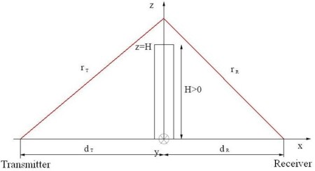
Figure 2. Transmitter and receiver scenario in knife edge model.
The transmitter is located at (-dT, 0, 0) and the receiver at (dR, 0, 0). A diffracting knife edge (semi plane) is located at x = 0 and has the height z = H. According to the principle of Huygens every point in the semi plane z > H can be considered as individual point source. The transmitter as point source provides a field strength F in the semi plane x = 0 according to the following formula:
to compute the field strength at the receiver location the principle of Huygens can be applied and accordingly every point above the absorbing semi plane can be considered as point source. The field strength at the receiver is computed as superposition of all fields provided by the point sources:
There are different modeling approaches for the determination of the knife edges between the transmitter and the receiver.
Approach According to Epstein and Peterson
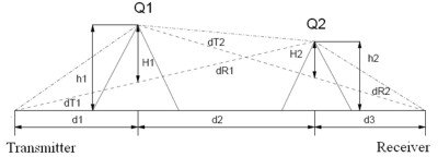
Figure 3. Knife edge model according to Epstein and Peterson.
Approach According to Deygout
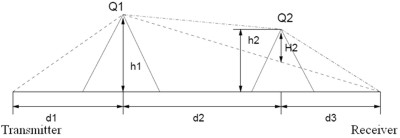
Figure 4. Knife edge model according to Deygout.