Exercise 2: Tensile Test of Elastomer
In this exercise, you will perform a uni-axial tensile test on a rubber strip (2mmx5mmx50mm).
Hyper-elastic material constants have been sourced from reference[3].
Hyper-elastic materials are large strain materials when compared to metals. In case of hyper-elastic materials the non-linear relation between stress and strain is derived from a strain energy density function. Currently MotionSolve supports three hyper-elastic material models: Neo-Hookean, Mooney–Rivlin, and Yeoh.
Add a New Material Property
In this step, you will add a new material property.
-
Click the Add button.
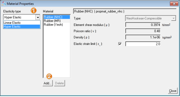
Figure 1. Adding new HyperElastic material -
For Source for values, select Rubber (Yeoh).
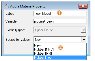
Figure 2. Selecting source values for new material -
In the Material Properties dialog, specify the material
constant values.
-
Element shear modulus (c10):
0.545235 -
Element shear modulus (c20):
0.0610498 -
Element shear modulus (c30):
−0.000802537 -
Poisson ratio (
 ):
): 0.48 -
Density (
 ):
): 1.1e-6 -
Elastic strain limit (εL):
2.0
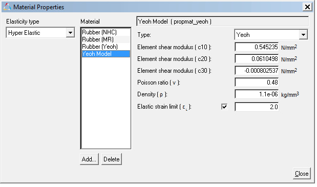
Figure 3. Specifying material constant values -
Element shear modulus (c10):
Model the Rubber Strip
In this step, you will model the rubber strip for the tensile test.
-
Use the
 (Create Points Along A Vector) macro to create 9
intermediate points between Rubber End 1 and Rubber end 2.
(Create Points Along A Vector) macro to create 9
intermediate points between Rubber End 1 and Rubber end 2.
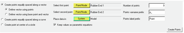
Figure 4. Creating intermediate points using “Create Points along a Vector” macro -
On the Model-Reference toolbar, click the
 (Body) icon.
-
Configure the Properties tab.
- Specify the Type as Beam.
- Specify the Cross-section as Bar.
-
For dim1, enter
2. -
For dim2, enter
25. - For the Material Property, select the Yeoh Model that you created previously.
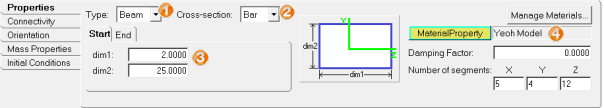
Figure 5. Specifying beam properties -
Configure the Connectivity tab.
-
Activate the first
 collector, and select the point
Rubber End 1.
collector, and select the point
Rubber End 1.
-
Select the next available intermediate points sequentially for the
other collectors, with the last collector being linked to
Rubber End 2.
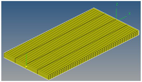
Figure 6. Rubber strip model
-
Activate the first
Add Constraints
In this step, you will create constraints for the rubber strip model.
-
In the Properties tab for the motion, for Define by: choose
Expression. In the Expression field, enter
`15*time`.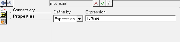
Figure 7. Motion expression -
On the Standard toolbar, click
 (Save Model) and save the model as
rubber_strip.mdlto your <working directory>.
Add Outputs
Now you will create outputs to measure engineering strain and engineering stress values.
Engineering Strain = 
Engineering Stress = 
-
Right-click the
 (Outputs) icon.
-
In the panel, for F2 type the expression
`(DM({j_trans.i.idstring},{j_fix.i.idstring})-50)/50`. For F3, type the expression`MOTION({mot_axial.idstring},{0},{2},{0})/50`.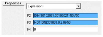
Figure 8. Output requestsNote: In the expression F2, the solver function DM() measures the distance magnitude between two markers; the I marker of the Translation Joint and the I marker of the Fix Joint. Expression F3 uses the solver function MOTION() which measures the reaction force due to the imposed motion Axial Motion.
Solve and Post-Process the Model
-
Click the
 (Run) panel icon.
-
After the simulation is completed, click Animate to view
the animation in HyperView.
You can use the
 (Start/Pause Animation) button
to play the animation.
(Start/Pause Animation) button
to play the animation. -
Go to the Contour panel, select NLFE Stress (t), XX and
click Apply.
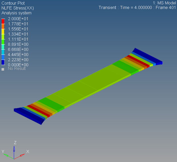
Figure 9. Stress contour -
Plot Engineering Stress vs Engineering Strain by selecting the data shown in
Table 4 and Table 5 in HyperGraph.
Table 4. X-Axis Data X Type Expression X Request REQ/70000000 Eng strain(F2), Eng Stress(F3) X Component F2 Table 5. Y-Axis Data Y Type Expression Y Request REQ/70000000 Eng strain(F2), Eng Stress(F3) Y Component F3 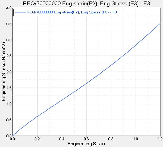
Figure 10. Stress versus strain curveNote: The animation shows the true stress due to cross-section deformation. -
Click to save the model.
-
Click
 and save the session as
hyperelastic.mvw.
References
JUSSI T, SOPANEN and AKI M. MIKKOLA:
Description of Elastic Forces in Absolute Nodal Coordinate Formulation. Journal of Nonlinear Dynamics 34: 53– 74, 2003.
Oleg Dmitrochenko:
Finite elements using absolute nodal coordinates for large deformation flexible multibody dynamics. Proceedings of the Third International Conference on Advanced Computational Methods in Engineering (ACOMEN 2005).
Sung Pil Jung, TaeWon Park, Won Sun Chung:
Dynamic analysis of rubber like material using absolute nodal coordinate formulation based on the non-linear constitutive law. Journal of Nonlinear Dyn (2011) 63: 149–157.