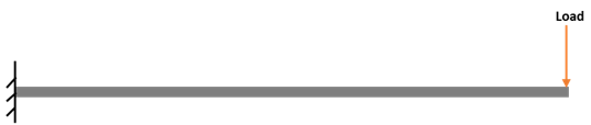
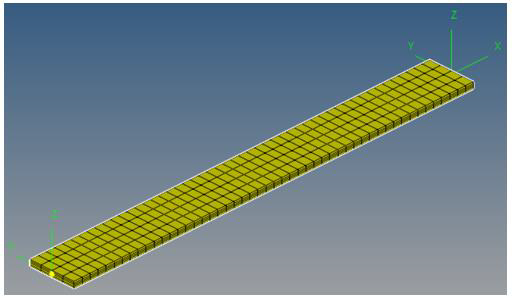
In this exercise, you will model a 1m long cantilever beam with a cross-section
dimension of 110mmx14mm to perform a bending test and compare it with an analytical
solution.
Before you begin, copy the
centerline.csv file, located in the
mbd_modeling\nlfe\intro folder, to your <working
directory>. Figure 1. Cantilever beam under end load condition
Model a Beam with Linear Elastic Material
In this step, you will model the cantilever beam with linear elastic
material.
Start a new MotionView session.
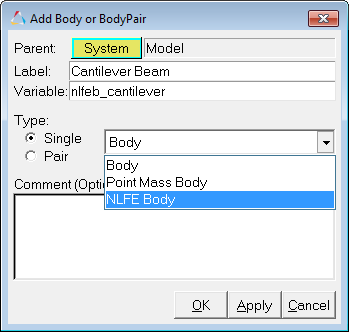
On the Reference toolbar, right-click on the (Body) icon.
In the Add Body or BodyPair dialog, specify the Label as
Cantilever Beam and the variable name as
nlfeb_cantilever.
In the drop-down menu, click NLFE Body. Then click
OK.
Figure 2.
This will display the NLFE Body with the Properties tab active.
Note:Table 1
shows the various tabs available in the NLFE Body panel.
Table 1.
Tab name
Sets NLFEBody
Properties
Type (Beam/Cable), Cross-section, and
materialproperties
Connectivity
Center line data or body profile
Orientation
Start and End orientations
Mass Properties
Displayed for information only
Initial Conditions
Initial velocities
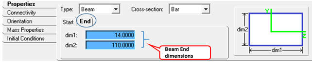
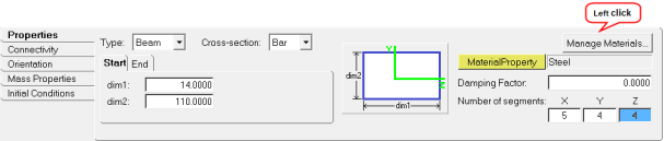
Configure the Properties tab.
For Type, choose Beam.
For Cross section: choose Bar.
For dim1, enter 14.0.
For dim2, enter 110.0.
The panel also displays the image of the cross-section indicating what
the different dimensions (dim1 and dim2) refer to.
Note: The Properties
tab has two sub-tabs called Start and End. These sub-tabs are used
to set the dimensions at two different ends of the beam. By default,
the End dimensions are parametrically equated to the Start
dimensions. If a different set of dimensions are provided at the
start and end, the cross section varies linearly along the length of
the beam.
Click the End sub-tab and review dim1 and dim2.
Figure 3.
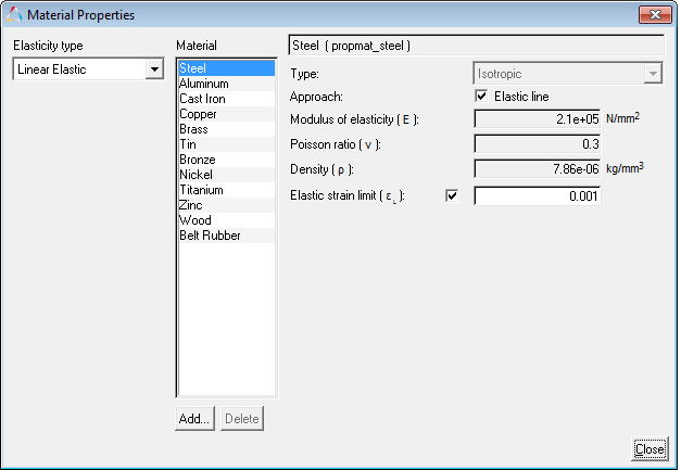
Click the Manage Materials button to display the
Material Properties dialog.
Figure 4.
Figure 5.
Tip: You can also access the Material
Properties dialog from the Model menu.
MotionSolve provides a list of commonly used Linear Elastic,
as well as Hyper Elastic material by default.
On the Materials list, choose Steel.
Review the property values and notice that the Elastic
line check box for Approach is selected.
Then click Close to close the dialog.
The default standard materials provided are defined with the Elastic Line
option checked on. Materials without the Elastic Line are solved using the
continuous mechanics approach, where in the cross-section deformation is taken
into consideration. The Elastic Line approach ignores cross-section deformation
effects, which gives results closer to an analytical solution.
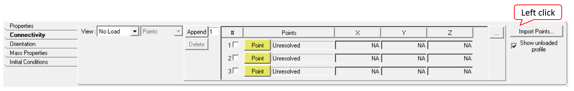
In the Connectivity tab, define the beam centerline by importing point data
from a CSV file. Click the Import Points button.
Figure 6.
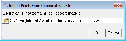
The Import Points From Coordinates In File dialog appears.
Browse to your <working directory> and choose the
centerline.csv file. Then click OK to import the points.
Figure 7.
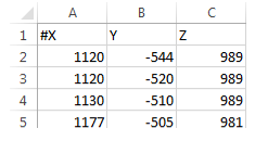
The .csv file must be in the following format: the first
column must hold the X-coordinates, the second column the Y-coordinates, and the
third column the Z-coordinates. There can also be a header row that begins with
a # indicating a commented line. Figure 8.
Press the 'F' key on your keyboard to fit the newly
created NLFE Body model to the modeling window.
Figure 9.
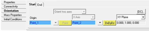
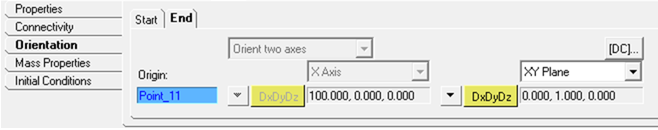
Click on the Orientation tab and review the Start and
End orientations.
Figure 10.
Figure 11.
Note: You can use the Orientation tab to set the cross section orientation (YZ
plane of the beam). Use the XY Plane or XZ Plane option to position the Y or
the Z-axis (the remaining axis will be positioned so that it is orthonormal
to the remaining two axes).
For this exercise, use the default orientations.
Intermediate Beam elements orientation is linearly varied from Start
orientation to End orientation. The Orientation option is useful in defining
twist along the beam length.
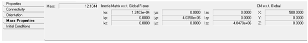
Click the Mass Properties tab to review the calculated
values.
Figure 12.
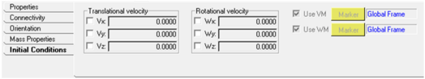
Click the Initial Conditions tab to review the NLFEBody
initial velocities.
Figure 13.
Leave initial velocities equal to zero.
Add a Constraint and Force
In this step, you will add a constraint and a force to the cantilever beam
model.
Create a fixed joint at the beam origin point (Point_1) using the specifics
shows in Table 2:
Table 2.
S. No
Label
Variable Name
Type
Body 1
Body 2
Origin(s)
Orientation Method
Reference 1
Reference 2
1
Fix Joint
j_fix
Fixed Joint
Cantilever Beam
Ground Body
Point_1
Note:
Each grid on an NLFE body has 12 DOFs: 3 translational, 3 rotational, and
6 related to the length and angle between the gradient vectors. Using a
fixed joint constrains the positions of the grid and the rigid body
rotations. However, the gradients at the grid are free. This means that
the cross-section at the fixed joint can twist about the grid and also
deform based on Poisson’s ratio. To arrest these DOFs, an NLFE element
called “CONN0” can be used.
There is no graphical user interface support for creating this
constraint. By default, MotionView creates a
CONN0 element at all of those grids of the NLFE body through which it is
attached to a constraint/force entity.
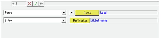
Create a load at the cantilever beam end point (Point_11) using the specifics
shown in Table 3:
Table 3.
S. No
Label
Variable
Force
Properties
Action force on
Apply force at
Ref. Marker
1
Load
frc_load
Action only
Scalar Force along Z axis of Ref Frame
Cantilever Beam
Point_11
Global Frame
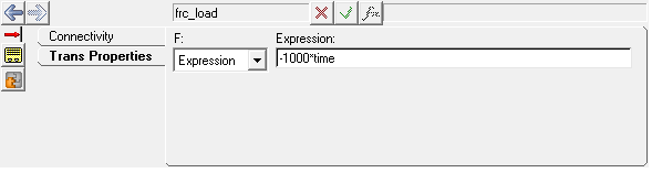
From the Trans Properties tab, specify the expression for force as `
-1000*time`.
Figure 14.
Note: Negative value is specified to apply load along negative Z-axis
direction.
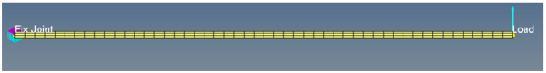
Figure 15. Cantilever beam with end load
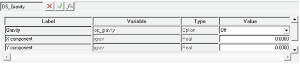
Turn off gravity to eliminate deflection due to beam self-weight.
Figure 16. Figure 17.
Create Outputs
In this step you will create outputs to measure cantilever beam end
deflection.
Cantilever beam end deflection from linear-elasticity theory:
Deflection for
load applied at end =
Where,
=
Load (N)
= Beam length = 1000mm
=
Youngs Modulus = 2.1e+05 N/mm2
=
Second Moment of Area = = 114 * =
25153.33mm4
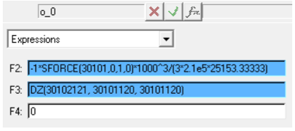
Right-click the (Outputs) button.
In the dialog, specify a label of Deflection - Analytical (F2),
NLFE(F3). Then click OK.
In the panel, specify the Type as Expressions.
In F2, enter
`-1*SFORCE({frc_load.idstring},0,1,0)*1000^3/(3*2.1e5*25153.33333)`.
For F3, enter `{frc_load.DZ}`.
Figure 18.
Click the (Check Model) button to check
the model for errors.
Add an output request Load.
This will measure the magnitude of the applied load. Figure 19.
Click and save the model as
nlfe_cantilever.mdl.
Solve and Post-Process the Model
Now you will solve the model with MotionSolve and view
the results.
Click the (Run) panel icon.
Specify the MotionSolve file name as
Cantilever_beam.xml.
Specify the Simulation type as Quasi-static, the End
time as 1 second, and the Print interval as
0.01.
Click the Run button.
After the simulation is complete, click the Animate
button to view the animation in HyperView.
You can use the (Start/Pause Animation) button
to play the animation.
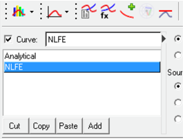
In the MotionView Run panel, click
Plot to load the .abf file in
HyperGraph.
Plot Deflection versus Load calculated from linear elasticity theory and NLFE
by selecting the data from Table 4 and Table 5 in HyperGraph.
In the panel, rename the two curves Analytical and
NLFE.
Figure 20. Define Curves panel
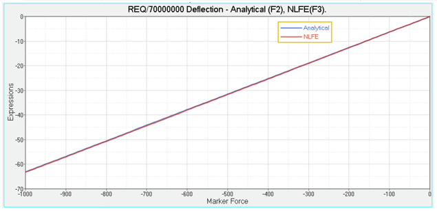
From the plot (shown in Figure 21), you can see that the two curves almost overlap. Figure 21. Deflection versus load plot
Click inside the HyperView animation window to make
it the active window.
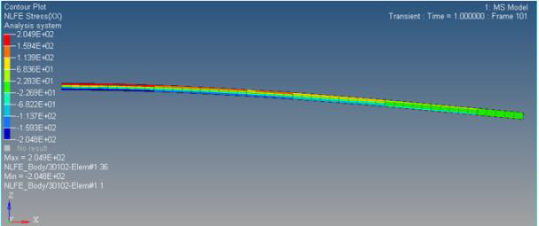
Click the (Contour) button to activate the
Contour panel.
Under Result type, select NLFE Stress (t) and
XX.
Click Apply.
This will show you the bending stress contours plot.
Note: You can also
view Displacement, Strain, etc. for an NLFE body in HyperView. All FE contours and types are available in
HyperView for an NLFE body. Figure 22. Bending stress contour of NLFE beam
Click and save the session as
nlfe_cantilever.mvw.
 (Body) icon.

 =
Load (N)
=
Load (N) = Beam length = 1000mm
 =
Youngs Modulus = 2.1e+05 N/mm2
=
Youngs Modulus = 2.1e+05 N/mm2 =
Second Moment of Area =
=
Second Moment of Area =  = 114 *
  =
25153.33mm4
=
25153.33mm4 (Outputs) button.
 (Check Model) button to check
the model for errors.
(Check Model) button to check
the model for errors.
 and save the model as
 (Run) panel icon.
 (Start/Pause Animation) button
to play the animation.
(Start/Pause Animation) button
to play the animation. (Define Curves) icon.
 (Contour) button to activate the
Contour panel.
(Contour) button to activate the
Contour panel.
 and save the session as