MV-2020: Use Flexbodies in MBD Models
In this tutorial, you will use the flexible bodies created in tutorial MV-2010 in an MBD model and solve the model using MotionSolve.
Integrate the Flexbodies into the MBD Model
In this exercise, you will integrate the flexbodies into your MBD model.
Set Up the Assembly Wizard
-
Select the Flex Body (CMS) check box and click
Yes to confirm both sides as deformable.
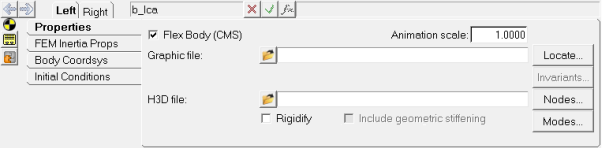
Figure 1.Notice that the graphics of the rigid body lower control arm vanishes.
-
Using the file browser
 select the file
sla_flex_left.h3d (created in earlier tutorial MV-2010)
from your working directory.
The H3D file field is populated automatically with the same path and the file name as the graphic file you specified earlier.
select the file
sla_flex_left.h3d (created in earlier tutorial MV-2010)
from your working directory.
The H3D file field is populated automatically with the same path and the file name as the graphic file you specified earlier.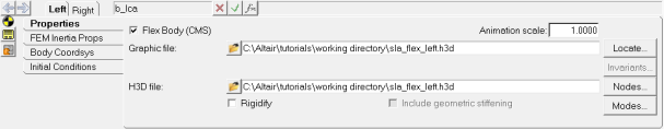
Figure 2. Properties PanelThe flexible body drops into the right position.
Note: You need to specify the flexbody H3D file as the H3D file. Specify the same or any other file as the graphic file.Use of large flexbodies is becoming very common. For faster pre-processing, you can use any graphic file for the display and use the flexbody H3D file to provide the data to the solver. You can use the input FEM deck or the CAD file used for the flexbody generation to generate a graphic H3D file using the CAD to H3D Conversion and specify that file as the graphic file. This will make pre-processing a much more efficient process.
Relocate the Flexbody
The Locate button on the Properties panel is an optional step to relocate a flexible body if it is not imported in the desired position. This may happen if the coordinate system used while creating the flexible body in the original FEM model does not match the MBD model coordinate system. However, if your flexible body is already in the desired position, you can skip this step.
-
Click Nodes.
The Nodes panel is displayed.
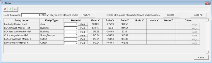
Figure 3.The Nodes panel is used to resolve the flexbody's attachments with the vehicle model, since the vehicle model is attached to the flexible body at these interface nodes.
This panel lists all markers of the connections (joints/forces) on the body which is now flexible. These markers can interact with the flexible body only through a node. This panel is used to map each of the markers to a node. The panel also displays the point coordinates of the marker origin which are nothing but coordinates of a point entity that the connections are referring to.
-
Click Modes.
The Modes panel is displayed. This option lets you select the modes that will be active during the simulation. By default, the rigid body modes are deactivated. You can also change the damping used for modes.
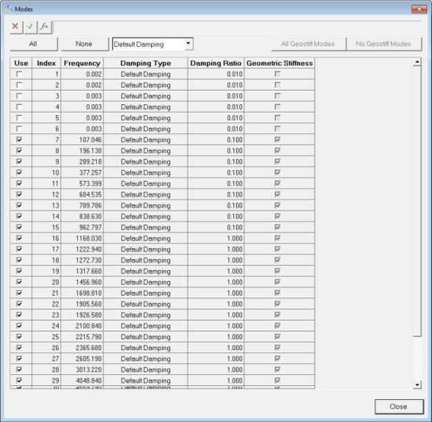
Figure 4.Please note that when selecting the modes, the simulation results may vary as you change the modes to be included in the simulation.
Note: By default, for frequencies under 100Hz, 1% damping is used. For frequencies greater than 100Hz and less than 1000Hz, 10% damping is used. Modes greater than 1000 Hz use critical damping. You can also give any initial conditions to the modes. -
Repeat steps 1 through 5 to integrate the right side flexible body
sla_flex_right.h3d (created in MV-2010: Flexbody Generation using Flex Prep and OptiStruct) in your model.
Your model should look like the image below:
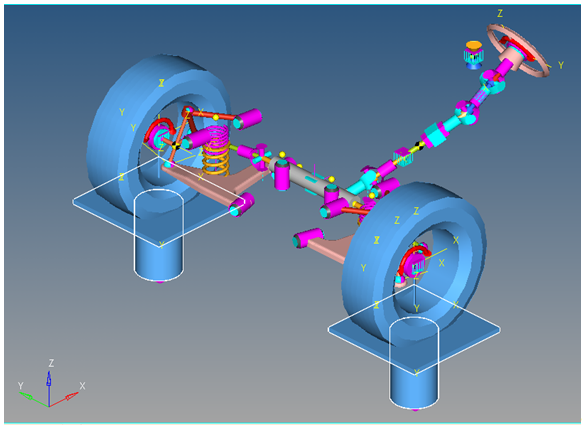
Figure 5.
Review the Properties of the FEM Model File
-
Click the FEM Inertia Props tab.
The following information is displayed:
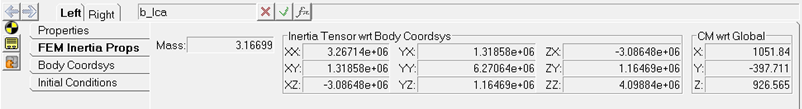
Figure 6. Bodies Panel/FEM Inertia Props Tab -
Click Run
 on the
toolbar and run the model with simulation type
Quasi-Static, specifying the filename as
sla_flex_ride.xml.
on the
toolbar and run the model with simulation type
Quasi-Static, specifying the filename as
sla_flex_ride.xml.