ACU-T: 3310 Single Phase Nucleate Boiling
Prerequisites
This tutorial introduces you to setting up and solving a single phase nucleate boiling problem using HyperMesh. Prior to starting this tutorial, you should have already run through the introductory tutorial, ACU-T: 1000 HyperWorks UI Introduction, and have a basic understanding of HyperMesh, AcuSolve, and HyperView. To run this simulation, you will need access to a licensed version of HyperMesh and AcuSolve.
Prior to running through this tutorial, copy HyperMesh_tutorial_inputs.zip from <Altair_installation_directory>\hwcfdsolvers\acusolve\win64\model_files\tutorials\AcuSolve to a local directory. Extract ACU-T3310_NB1.hm from HyperMesh_tutorial_inputs.zip.
Since the HyperMesh database (.hm file) contains meshed geometry, this tutorial does not include steps related to geometry import and mesh generation.
Problem Description

Figure 1. Schematic of Channel
The dimensions of the inlet are 0.03 x 0.04 m; the inlet velocity (v) is 0.39 m/s and the temperature (T) of the fluid entering the inlets is 368.15 K (95 C).
The preheated air enters the inlets and heat is transferred to the fluid from the walls. The heat causes sub-cooled boiling to occur in the region close to the wall and leads to formation of bubbles at nucleation sites.
The heat transfer in this regime is basically dominated by two effects, the macro convection due to the motion of the bulk liquid and the latent heat transport associated with the evaporation of the liquid micro-layer between the bubble and the heated wall.
The fluid in this problem is water, which has temperature dependent material properties: density, viscosity, enthalpy and conductivity. There are also surface tension and vapor phase models specified for this material.
Water vapor which also has temperature dependent material properties is specified as the vapor phase model.
The AcuSolve simulation will be set up to model steady state heat transfer to determine the temperature and heat flux on the heated walls of the manifold.
Open the HyperMesh Model Database
-
Click the Open Model icon
 located on the standard toolbar.
The Open Model dialog opens.
located on the standard toolbar.
The Open Model dialog opens.
Set the Simulation Parameters
Set the General Simulation Parameters
-
Set Nucleate boiling single phase to On.
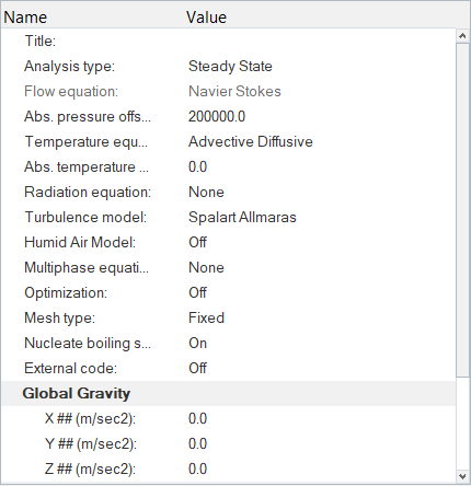
Figure 2.
Specify the Solver Settings
- In the Solver Browser, click 02.SOLVER_SETTINGS under 01.Global.
- In the Entity Editor, set the Relaxation factor to 0.4.
- Verify that Flow, Temperature, and Turbulence are set to On.
Set the Nodal Initial Conditions
-
Set a constant Eddy viscosity value of 0.0001.
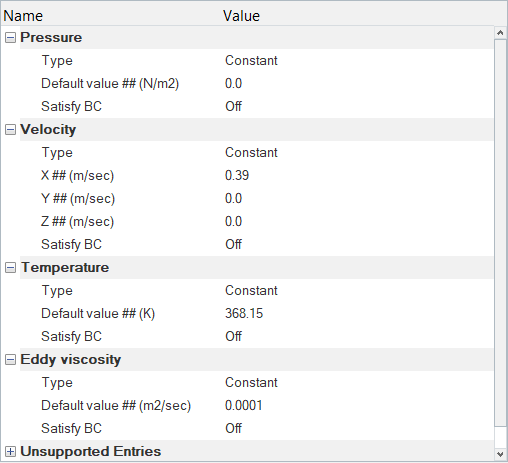
Figure 3.
Assign Material Properties and Boundary Conditions
Create Curves/Plots for Material Properties
-
Enter the X and Y values shown below.
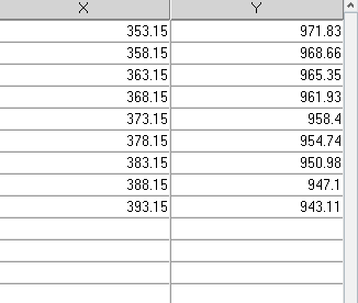
Figure 4. -
Create another curve, name it Viscosity_Water, and enter
the values shown below.
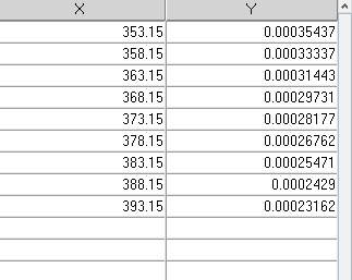
Figure 5. -
Create a curve named Enthalpy_Water and enter the
following values
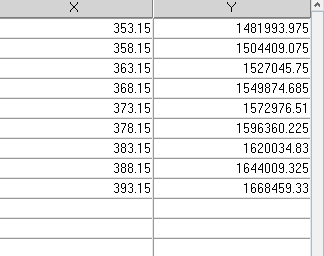
Figure 6. -
Create a curve named Conductivity_Water and enter the
following values.
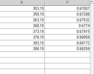
Figure 7. -
Create a curve named Density_Vapor and enter the
following values.
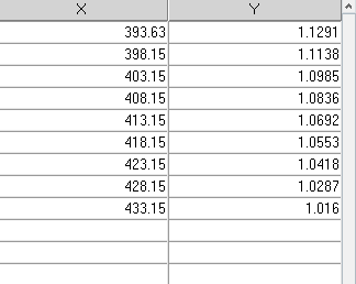
Figure 8. -
Create a curve named Viscosity_Vapor and enter the
following values.
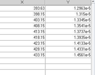
Figure 9. -
Create a curve named Enthalpy_Vapor and enter the
following values.
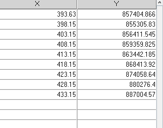
Figure 10. -
Create a curve named Conductivity_Vapor and enter the
following values.
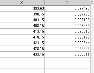
Figure 11. -
Set the value of the surface tension to 0.01.
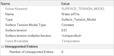
Figure 12.
Define Material Properties
-
Similarly for Viscosity and Conductivity, set the cubic spline values to
Viscosity_Vapor and
Conductivity_Vapor, respectively.
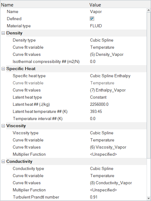
Figure 13. -
Similarly for Specific Heat, Viscosity, and Conductivity, set the cubic spline
values to Enthalpy_Water
Viscosity_Water and
Conductivity_Water, respectively.
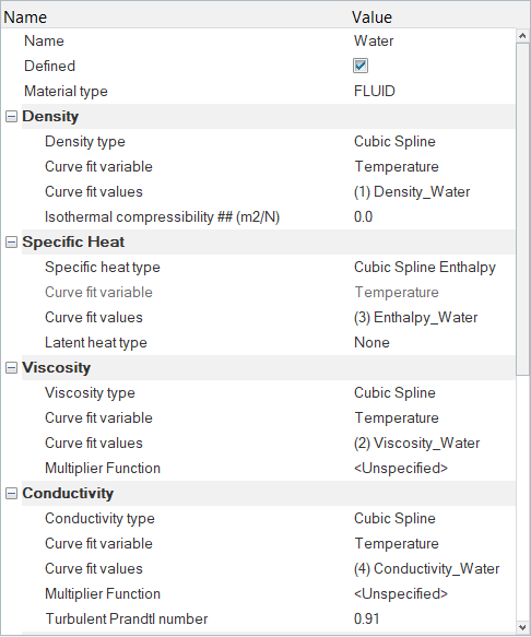
Figure 14. -
Under the Surface Tension heading, set the Surface tension model to
Water-srfTns by selecting it from the Plot
list.
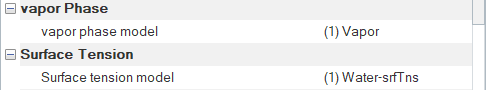
Figure 15.
Assign Material Properties and Boundary Conditions
-
Click FluidVolume. In the Entity Editor,
- Verify that the Type is set to FLUID.
- Select Water as the Material.
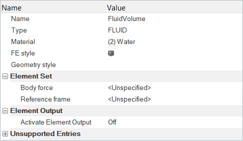
Figure 16. -
Click Inflow. In the Entity Editor,
- Change the Type to INFLOW.
- Set the Inflow type to Average Velocity.
- Set the Average velocity to 0.39 m/sec.
- Set the Temperature to 368.15 K.
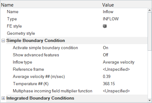
Figure 17. -
Click Outflow. In the Entity Editor,
- Change the Type to OUTFLOW.
- Verify that the Pressure value is set to 0 N/m2.
- Turn on the Backflow conditions and set the Temperature backflow type and Eddy viscosity backflow type to Mass Flux Average.
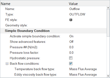
Figure 18. -
Click HeatedWall. In the Entity Editor,
- Verify that the Type is set to WALL.
- Set the Temperature BC Type to Value.
- Set the Temperature to 403.15 K.
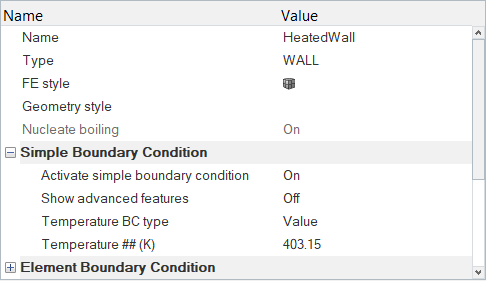
Figure 19.
Compute the Solution
-
Click
 on the ACU toolbar.
The Solver job Launcher dialog opens.
on the ACU toolbar.
The Solver job Launcher dialog opens. -
Leave the remaining options as
default and click Launch to start the solution
process.
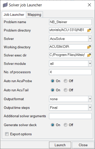
Figure 20.Once you hit the Launch button, the AcuTail and AcuProbe windows are launched automatically. A summary of the run in the AcuTail window indicates that the solver run is complete.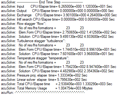
Figure 21.Once the run is complete, you can close the AcuTail and AcuProbe windows.
Post-Process the Results with HyperView
Once the AcuSolve run is complete, close the HyperWorks Solver View dialog. In the HyperMesh Desktop window, close the AcuSolve Control and Solver job Launcher dialogs. In the next few steps, you will plot a contour of temperature on the Heated Wall and Bottom surfaces.
Switch to the HyperView Interface and Load the AcuSolve Model and Results
-
In the HyperMesh Desktop window, click the
ClientSelector drop-down in the bottom-left corner of
the graphics window.
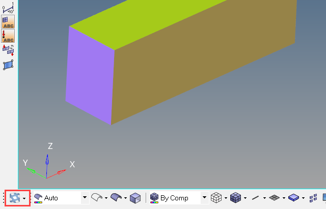
Figure 22. -
In the Load model and results panel, click
 next
to Load model.
next
to Load model.
Create Contours for Temperature Distribution
-
Click the Isolate Shown icon
 , hold Ctrl, then select the
HeatedWall and Bottom
components to turn off the display of all components except those that are
required.
, hold Ctrl, then select the
HeatedWall and Bottom
components to turn off the display of all components except those that are
required.
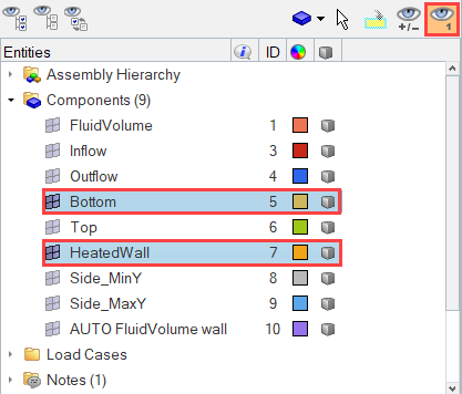
Figure 23. -
Click
 on the Results toolbar to open the Contour panel.
-
In the panel area, under the Display tab, turn off the
Discrete color option.
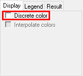
Figure 24.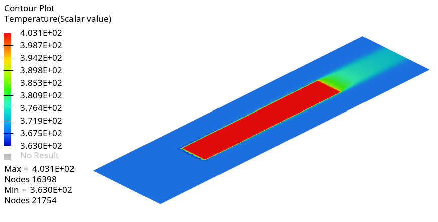
Figure 25.