ACU-T: 3000 Enclosed Hot Cylinder: Natural Convection
Prerequisites
This tutorial provides instructions for setting up, solving and viewing results of a CFD simulation of air flow inside the annulus of a concentric cylinder with a heat source due to natural convection. Prior to starting this tutorial, you should have already run through the introductory tutorial, ACU-T: 1000 HyperWorks UI Introduction, and have a basic understanding of HyperMesh, AcuSolve, and HyperView. To run this simulation, you will need access to a licensed version of HyperMesh and AcuSolve.
Prior to running through this tutorial, copy HyperMesh_tutorial_inputs.zip from <Altair_installation_directory>\hwcfdsolvers\acusolve\win64\model_files\tutorials\AcuSolve to a local directory. Extract ACU-T3000_HotCylinder.hm from HyperMesh_tutorial_inputs.zip.
Since the HyperMesh database (.hm file) contains meshed geometry, this tutorial does not include steps related to geometry import and mesh generation.
Problem Description

Figure 1.
The schematic of the problem to be solved is shown in the figure above. The inner cylinder is a solid with internal heat generation and the annular space between the inner and outer cylinders is a fluid volume with air as the fluid. The air in contact with the surface of the inner cylinder is heated up and rises to the upper parts of the annulus due to buoyancy effects and displaces the cold fluid at the top. At the same time, the film of the fluid which was in contact with the hot surface is replaced by the surrounding cold fluid. This process is repeated continuously until a steady state is achieved.
Both cylinders are assumed to be infinitely long and are modeled using half symmetry and periodicity. The cylinders are infinite in z-direction and hence periodicity will be applied along this direction.
Introduction to Theory
Natural Convection
Convection is a heat transfer mechanism where the transfer of heat energy happens through the motion of matter. Since the definition of convection involves motion of matter a fluid state is usually present in convection. Usually this type of heat transfer takes place between a hot or a cold surface and a fluid. The film of fluid in contact with the surface absorbs heat from or transfers heat to the surface and is then replaced by a new film. This movement of fluid may either be governed by an external source, such as a fan or pump, or due to internal changes in the fluid properties. When no external sources are responsible for the fluid motion the heat transfer mechanism at work is called the Natural Convection. The driving force for motion of the fluid in a natural convection is density changes in the fluid due to temperature gradients induced in the fluid by heat transfer.
The natural convection mechanism works similarly as described above, whilst discussion of the problem. The fluid which is in contact with the surface absorbs or transfers heat from the surface and becomes hotter or colder than the surrounding fluid. Driven by buoyancy forces due to difference in densities caused by the temperature gradient, the fluid is displaced upwards or downwards. Surrounding fluid fills in the void created by the displaced fluid, which then undergoes the same process again. This gives rise to a convection current which drives the hot fluid to the top and cold fluid to the bottom of the convection cell. Buoyancy effects are driven by gravity, therefore natural convection requires presence of a gravitational force to work. It must be noted, however, that gravity is not the driving force behind the fluid movement. Presence of gravity only enables displacement of the fluid due to the density changes caused by temperature gradients.
Mathematical determination of the onset of natural convection is done through a dimensionless number called the Rayleigh number (Ra). The Rayleigh number is defined as:
- x is the characteristic length (m)
- is the Rayleigh number for characteristic length x
- is acceleration due to gravity (m/s2)
- is the surface temperature (K)
- is the quiescent temperature (fluid temperature far from the surface of the object) (K)
- is the kinematic viscosity (m2/s)
- α is the thermal diffusivity (m2/s)
- β is the thermal expansion coefficient (equals to for ideal gases where is absolute temperature).
The fluid properties , α and β are evaluated at the film temperature, , which is defined as:
When the Rayleigh number is below a critical value for the fluid heat transfer is primarily in the form of conduction. When it exceeds this critical value the dominant heat transfer mechanism is convection.
Boussinesq Density Model
The Boussinesq density model is an approximation method applied to buoyancy driven flows, such as natural convection flows. In the Boussinesq approximation, the density variation terms are neglected everywhere except when multiplied by acceleration due to gravity, . The basis of this approximation is that since temperature changes are small, the resultant changes in density are small as well and thus can be neglected. However, when multiplied by , the resultant term gives rise to forces which no longer are negligible. The Boussinesq approximation is:
- is the instantaneous density at temperature (kg/m3)
- is the density at reference temperature (kg/m3)
- is change in temperature (K)
As stated in the approximation, the Boussinesq density model is only applicable when density variations are small. A general guideline is to check for the condition to be true. This indirectly puts a limitation on this model to be used to only for cases where expected temperature differences within the fluid are not large.
Open the HyperMesh Model Database
-
Click the Open Model icon
 located on the standard toolbar.
The Open Model dialog opens.
located on the standard toolbar.
The Open Model dialog opens.
Set the General Simulation Parameters
Set the General Simulation Parameters
-
Set the Temperature equation to Advective
Diffusive.
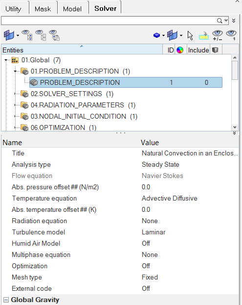
Figure 2.
Specify the Solver Settings
-
Turn On Temperature flow.
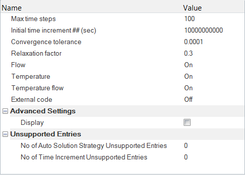
Figure 3.
Create Time History Output Points
The Time History Output command enables you to extract the nodal solution at any point within the domain.
-
Click
 to open the No of Coordinates
dialog. In the dialog, enter the values as shown in the figure below then close
the dialog.
to open the No of Coordinates
dialog. In the dialog, enter the values as shown in the figure below then close
the dialog.
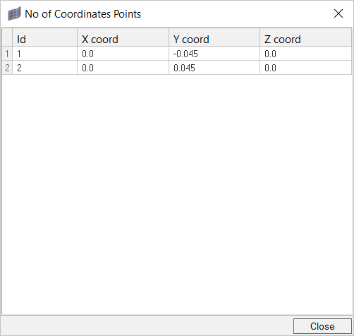
Figure 4. -
Set the Output frequency to 1.
By setting this, the surface output is written for each time step at the specified coordinate points.
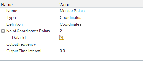
Figure 5.
Set the Body Force and Material Model Parameters
Modify the Material Model Parameters of Air
-
Verify that the Expansivity and Reference temperature values are set to
0.00347222222222 K-1 and
288 K respectively.
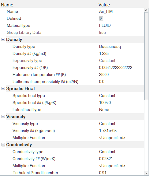
Figure 6.
Create a Material Model for the Solid
-
Set the Conductivity value to 16.2 W/m-K.
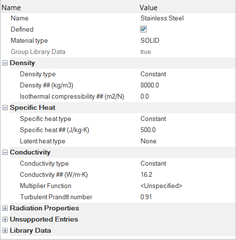
Figure 7.
Define the Gravitational Body Force
-
Change the Z Gravity to 0.
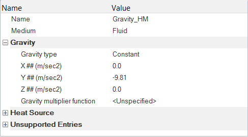
Figure 8.
Define the Volumetric Heat Source
-
Set the Volumetric heat source value to 20000
W/m3.
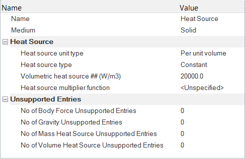
Figure 9.
Specify the Boundary Conditions and Initial Conditions
Specify the Material Properties and Surface Boundary Conditions
-
Click Solid. In the Entity Editor,
- Change the Type to SOLID.
- Select Stainless Steel as the Material.
- Set the Body force to Heat Source.
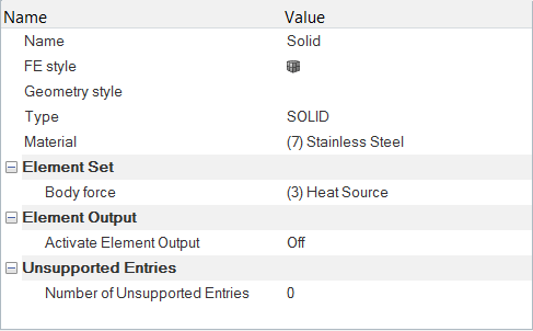
Figure 10. -
Click Fluid. In the Entity Editor,
- Change the Type to FLUID.
- Select Air_HM as the Material.
- Set the Body force to Gravity_HM.
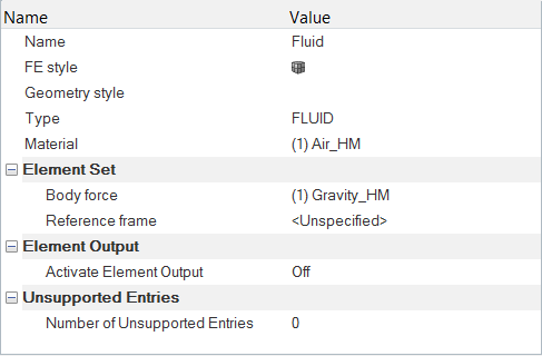
Figure 11. -
Click solid_pos_z. In the Entity Editor, turn Off the simple
boundary condition.
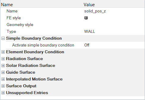
Figure 12. -
Click symmetry. In the Entity Editor, change the Type to
SYMMETRY.
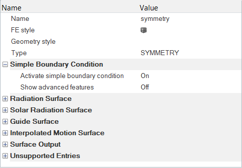
Figure 13. -
Click inner_wall. In the Entity Editor, verify that the Type is set to
WALL.
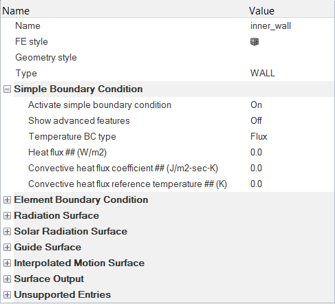
Figure 14. -
Click outer_wall. In the Entity Editor,
- Verify that the Type is set to WALL.
- Change the Temperature BC type to Value.
- Set the Temperature to 298 K.
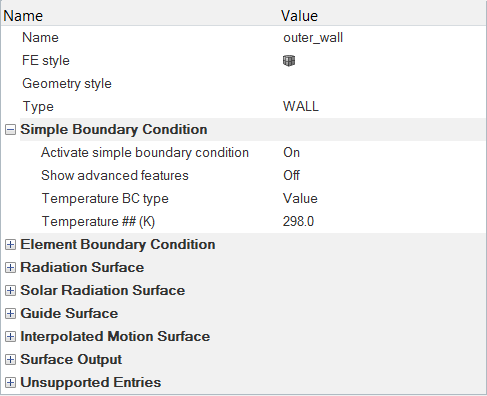
Figure 15.
Specify the Periodic Boundary Conditions
Since you are modeling only a portion of the infinitely long domain, you need to define the periodicity of the solution by specifying periodic boundary conditions. The solution is then constrained by periodicity. The periodic boundary condition links the corresponding pairs of nodes on the two surfaces on which the periodicity is defined.
-
Similarly, set the Target component to
fluid_neg_z.
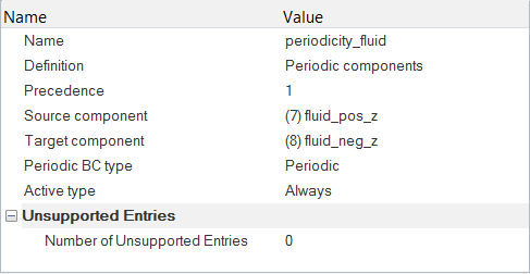
Figure 16.
Specify the Reference Pressure
Since this model set up doesn’t have an inlet and outlet, we need to specify the reference pressure manually. This can be done by specifying a pressure nodal boundary condition at a node in the fluid region.
-
Click the Node entity collector then pick a node in the
fluid region from the modeling window.
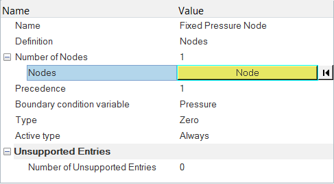
Figure 17.
Specify the Nodal Initial Conditions
-
In the Entity Editor, set the Default value for
Temperature to 353.15 K.
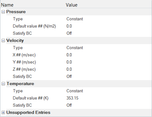
Figure 18.
Compute the Solution
-
Click
 on the ACU toolbar.
The Solver job Launcher dialog opens.
on the ACU toolbar.
The Solver job Launcher dialog opens. -
Leave the remaining options as
default and click Launch to start the solution
process.
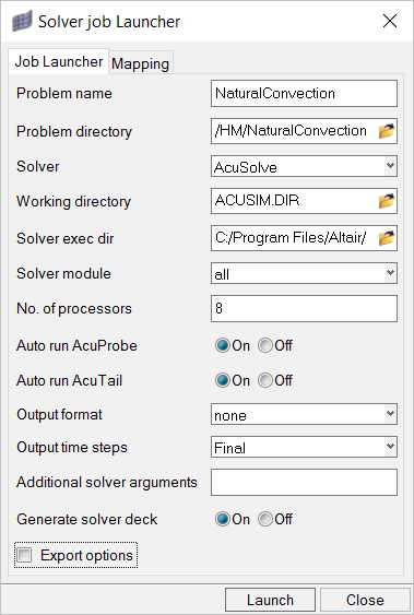
Figure 19.
Post-Process the Results
As the solution progresses, the AcuProbe and AcuTail windows are launched automatically. The progress of the solution can be monitored using these applications.
Post-Process with AcuProbe
-
Similarly, expand node 2, right-click on
temperature, and select
Plot.
The temperature plot at both the locations should be displayed in the plot window as shown below.Note: You might need to click
 on the toolbar in order to
properly display the plot.
on the toolbar in order to
properly display the plot.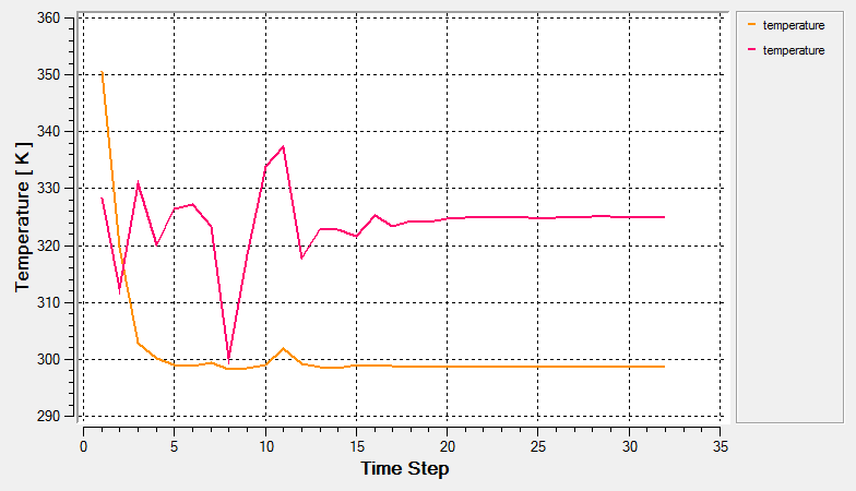
Figure 20.
Open HyperView and Load the Model and Results
-
In the Load model and results panel, click
 next
to Load model.
next
to Load model.
Create a Temperature Distribution Contour
-
Click
 on the Results toolbar to open the Contour panel.
-
Orient the display to the xy-plane by clicking
 on the Standard Views toolbar.
-
In the panel area, under the Display tab, turn off
the Discrete color option.
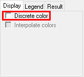
Figure 21. -
Click the Legend tab then
click Edit Legend. In the dialog, change the Numeric
format to Fixed then click
OK.
Verify that the contour plot looks like the figure shown below.
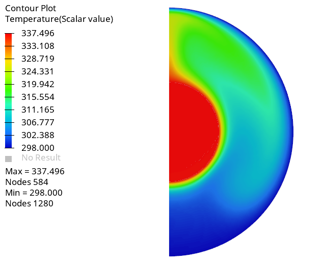
Figure 22.
Create a Velocity Vector Plot
-
Click
 on the Results toolbar to open the Vector panel.
-
Click Apply in the panel area.
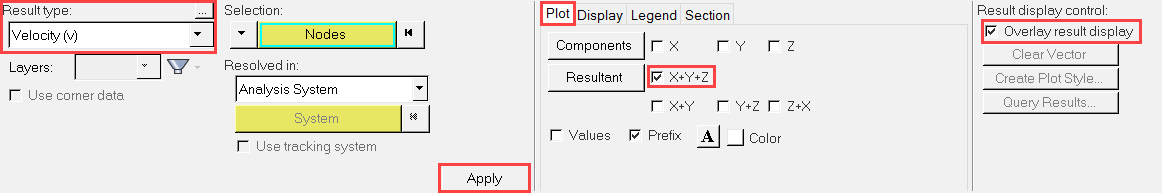
Figure 23. -
Set the Vector heads options to Arrow and
Tip.
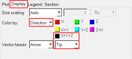
Figure 24.The Vector plot should be modified accordingly as you make the changes mentioned above. Verify that the vector plot looks like the one shown in the figure below. The plot is zoomed in for a clear display of the direction of air flow.
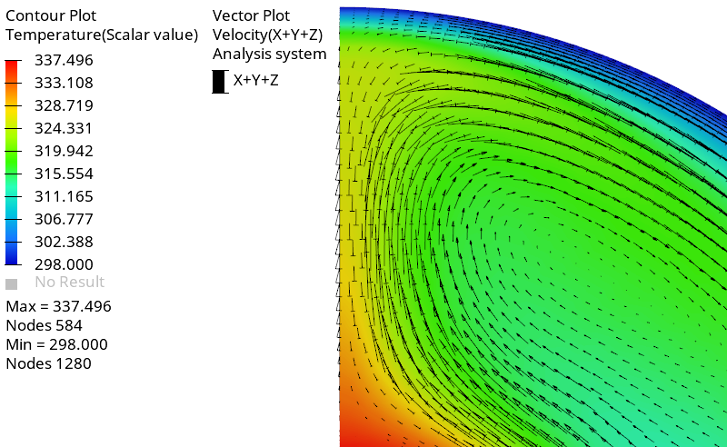
Figure 25.As mentioned in the problem description, the air which is in contact with the solid surface gets heated up and rises to the top while being replaced by the colder air and the cycle gets repeated until steady state is reached.
Summary
In this tutorial, you successfully learned how to set up and solve a natural convection problem using AcuSolve in HyperMesh. You started by importing the HyperMesh model database and then set up the simulation parameters and boundary conditions. Once the solution was computed, you post-processed the results using HyperView and created a contour plot of temperature distribution across the domain.