ACU-T: 3204 Radiation Heat Transfer in a Simple Headlamp using the Discrete Ordinate Model
Prerequisites
This tutorial introduces you to setting up a radiation heat transfer problem using the Discrete Ordinate radiation model in HyperMesh and solving using AcuSolve. Prior to starting this tutorial, you should have already run through the introductory tutorial, ACU-T: 1000 HyperWorks UI Introduction, and have a basic understanding of HyperMesh, AcuSolve, and HyperView. To run this simulation, you will need access to a licensed version of HyperMesh and AcuSolve.
Prior to running through this tutorial, copy HyperMesh_tutorial_inputs.zip from <Altair_installation_directory>\hwcfdsolvers\acusolve\win64\model_files\tutorials\AcuSolve to a local directory. Extract ACU-T3204_HeadlampDO.hm from HyperMesh_tutorial_inputs.zip.
Since the HyperMesh database (.hm file) contains meshed geometry, this tutorial does not include steps related to geometry import and mesh generation.
Problem Description

Figure 1.
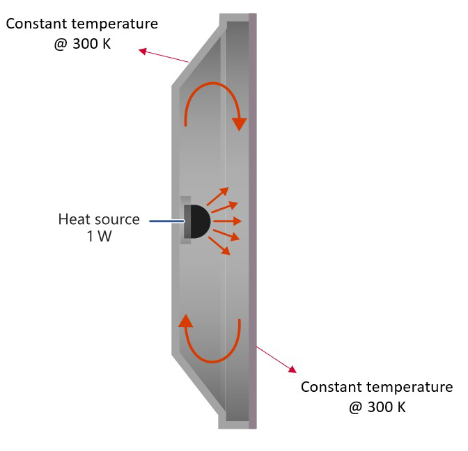
Figure 2.
| Absorption Coefficient | Refractive Index | |
|---|---|---|
| Air | 0 | 1.0 |
| Lens | 900 | 1.57 |
| Surface Type | Radiation Surface Type |
|---|---|
| Participating medium - Participating medium Interface | Radiation Interface - Internal |
| Participating medium - (Non- Participating) medium Interface | Wall |
| External boundaries of Participating medium | Radiation Interface - External or Wall |
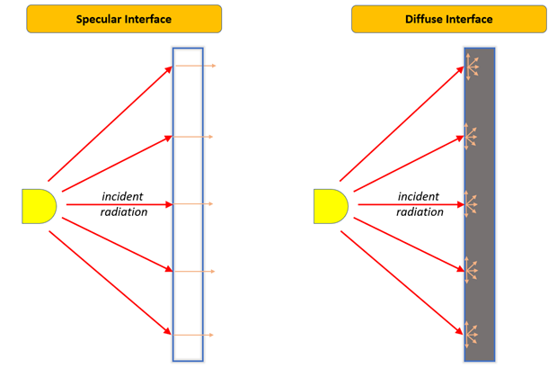
Figure 3.
Open the HyperMesh Model Database
-
Click the Open Model icon
 located on the standard toolbar.
The Open Model dialog opens.
located on the standard toolbar.
The Open Model dialog opens.
Set the General Simulation Parameters
Set the Analysis Parameters
-
Set the Turbulence model to Laminar (if not set
already).
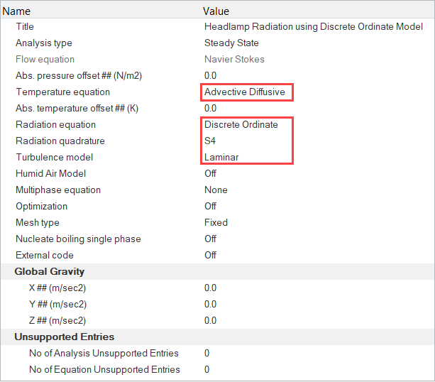
Figure 4.
Specify the Solver Settings
-
Leave the remaining options unchanged.
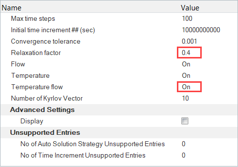
Figure 5.
Define the Material Models and the Body Force
Define the Material Models
-
Set the Absorption coefficient to 0 and Refractive index
to 1.
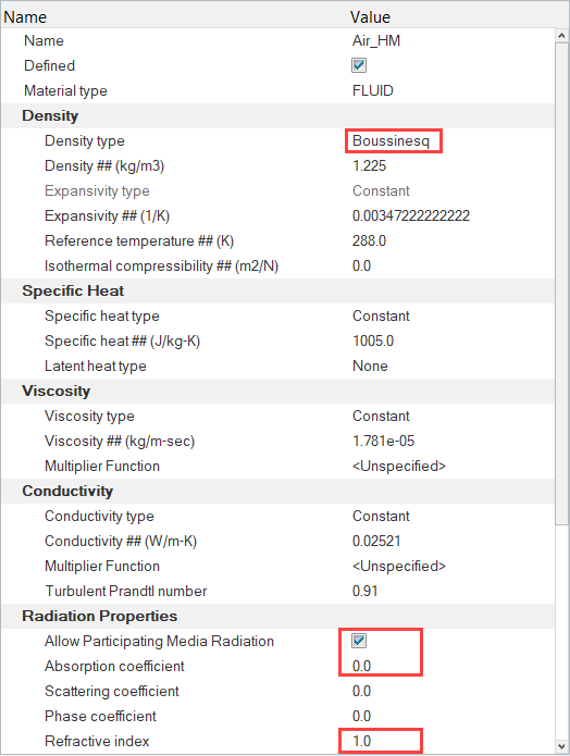
Figure 6. -
Set the Absorption coefficient to 900 and the Refractive
index to 1.57.
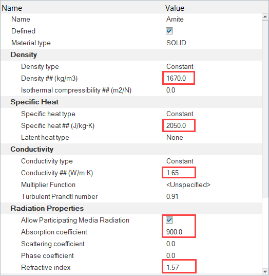
Figure 7.
Define the Body Force
-
In the Entity Editor, set the Y-Gravity to
-9.81 m/sec2 and change to Z-Gravity to
0.
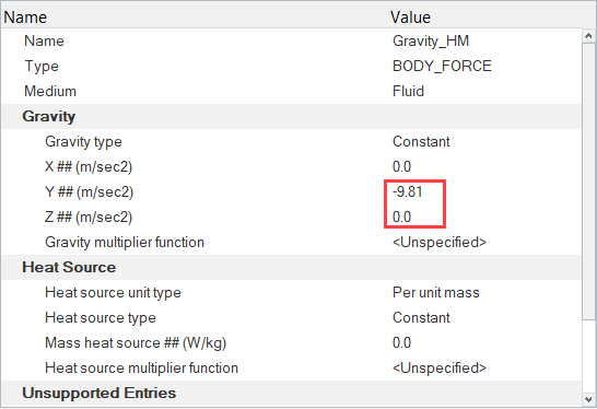
Figure 8.
Define the Heat Source
-
Set the Heat Source type to Constant and set the
Volumetric heat source to 2049180 W/m3.
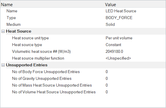
Figure 9.
Set the Boundary Conditions
Create the Emissivity Model
- In the Solver Browser, right-click on 07.Emissivity_Model and select Create.
- In the Entity Editor, name it Inner.
- Set the Emissivity to 0.05.
Set the Boundary Conditions
-
Click Air. In the Entity Editor,
- Change the Type to FLUID.
- Set the Material to Air_HM.
- Set the Body force to Gravity_HM.
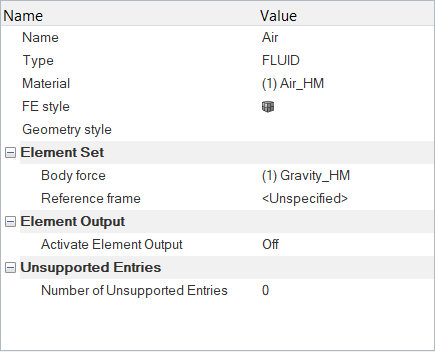
Figure 10. -
Click Housing. In the Entity Editor,
- Change the Type to SOLID.
- Set the Material to Plastic.
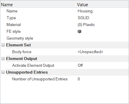
Figure 11. -
Click Bulb. In the Entity Editor,
- Change the Type to SOLID.
- Set the Material to LED.
- Set the Body force to LED Heat Source.
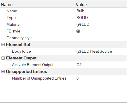
Figure 12. -
Click Lens. In the Entity Editor,
- Change the Type to SOLID.
- Set the Material to Arnite.

Figure 13. -
Click Lens-inner. In the Entity Editor, verify that the Type is set to
WALL. Under the Radiation Surface tab,
- Activate the Display checkbox and set the Active radiation surface field to On.
- Set the Type to Radiation Interface and the Radiation interface type to Internal.
- Set the Diffused fraction to 0.
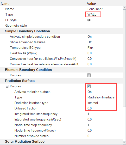
Figure 14. -
Click Lens-outer. In the Entity Editor, verify that the Type is set to
WALL. Set the Temperature BC type to
Value and set the Temperature to
300 K. Under the Radiation Surface tab,
- Activate the Display checkbox and set the Active radiation surface field to On.
- Set the Type to Radiation Interface and the Radiation interface type to External.
- Set the External emissivity model to Black Body.
- Set the External refractive index to 1 and the External temperature to 300 K.
- Set the Diffused fraction to 1.
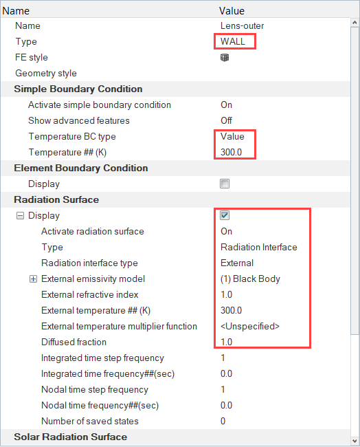
Figure 15. -
Click Housing-Lens-interface. In the Entity Editor, verify that the Type is set to
WALL. Under the Radiation Surface tab,
- Activate the Display checkbox and set the Active radiation surface field to On.
- Set the Type to Wall and the Emissivity model to Black Body.
- Set the Diffused fraction to 1.
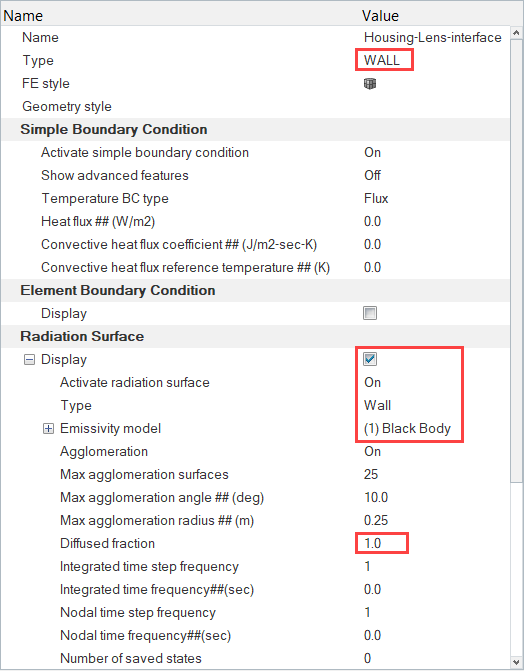
Figure 16. -
Click Housing-inner. In the Entity Editor, verify that the Type is set to
WALL. Under the Radiation Surface tab,
- Activate the Display checkbox and set the Active radiation surface field to On.
- Set the Type to Wall and the Emissivity model to Inner.
- Set the Diffused fraction to 1.
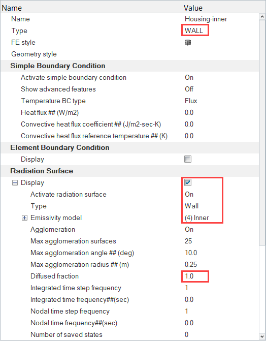
Figure 17. -
Click Housing-outer. In the Entity Editor,
- Verify that the Type is set to WALL.
- Set the Temperature BC type to Value.
- Set the Temperature to 300 K.
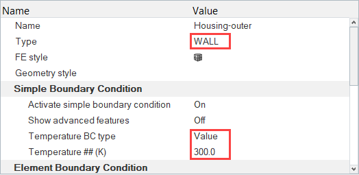
Figure 18. -
Click Bulb_walls. In the Entity Editor, verify that the Type is set to
WALL. Under the Radiation Surface tab,
- Activate the Display checkbox and set the Active radiation surface field to On.
- Set the Type to Wall and the Emissivity model to Black Body.
- Set the Diffused fraction to 1.
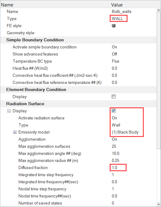
Figure 19.
Compute the Solution
Run AcuSolve
In this step, you will launch AcuSolve to compute a solution for this case.
-
Click
 on the ACU toolbar.
The Solver job Launcher dialog opens.
on the ACU toolbar.
The Solver job Launcher dialog opens. -
Leave the remaining options as
default and click Launch to start the solution
process.
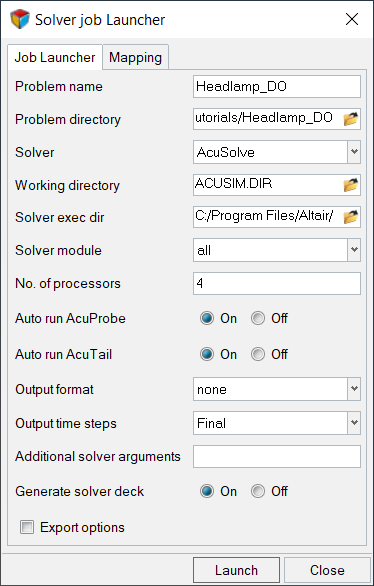
Figure 20.
Monitor the Solution with AcuProbe
While AcuSolve is running, you can monitor the progress of the solution using AcuProbe and plot the values of residual ratios, solution ratios, and variables like temperature, heat flux, etc. Once the solver run has started, the AcuTail and AcuProbe windows should be launched automatically.
-
Right-click on All and select Plot
All.
Note: You might need to click
 on the toolbar in order to
properly display the plot.
on the toolbar in order to
properly display the plot.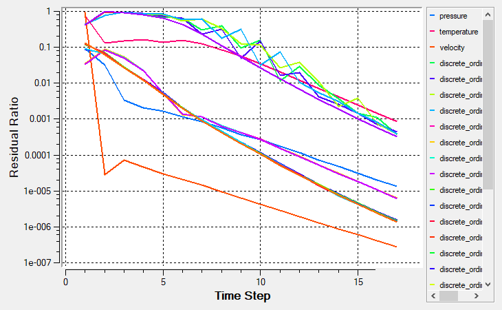
Figure 21.
Post-Process the Results with HyperView
In this step, you will visualize the results using HyperView. While doing so, you will create contour plots of temperature and incident radiation on a section cut. Once the solver run is complete, close the AcuProbe and AcuTail windows. In the HyperMesh Desktop window, close the AcuSolve Control tab and save the model.
Switch to the HyperView Interface and Load the AcuSolve Model and Results
-
In the HyperMesh Desktop window, click the
ClientSelector drop-down in the bottom-left corner of
the graphics window.
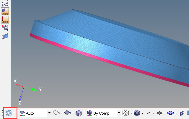
Figure 22. -
In the Load model and results panel, click
 next
to Load model.
next
to Load model.
Create Temperature and Incident Radiation Contours on a Section Cut
-
Orient the display to the xy-plane by clicking
 on the Standard Views toolbar.
-
On the 3DViewControls toolbar, right-click on
 multiple times until the orientation of the model is as
shown in the figure below.
multiple times until the orientation of the model is as
shown in the figure below.
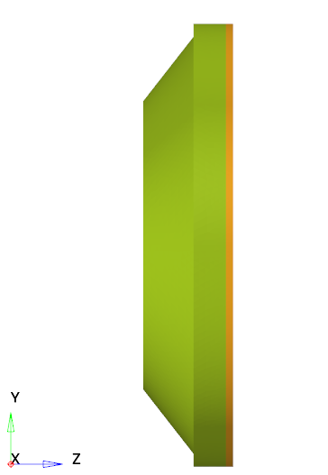
Figure 23. -
Click the Section cut icon
 on the HV-Display toolbar.
-
Change the Display options from Clipping plane to Cross
section.
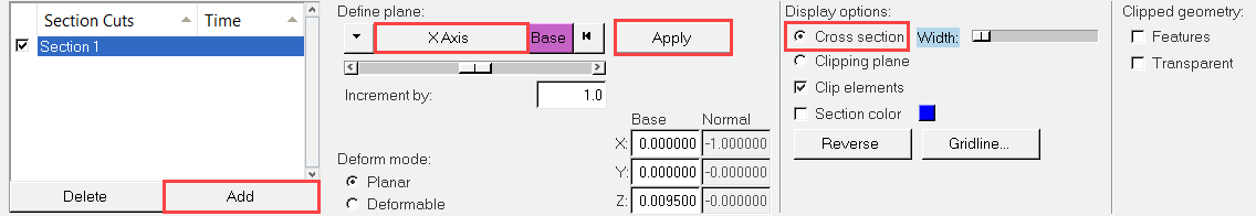
Figure 24. -
Click
 on the Results toolbar to open the Contour panel.
-
In the panel area, under the Display tab, turn off
the Discrete color option.
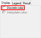
Figure 25. -
Click the Legend tab then click Edit
Legend. In the dialog, change the Numeric precision to
2 then click OK.
The contour plot should look like the one shown in the figure below.
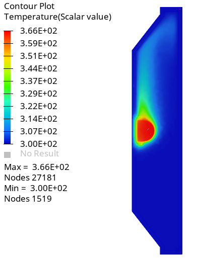
Figure 26. -
In the panel area, change the Result type to
Incident_radiation then click
Apply.
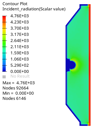
Figure 27.As seen in the figure above, the rays travel from the bulb through the air and lens before getting radiated to the atmosphere.
Summary
In this tutorial, you learned how to set up and solve a radiation heat transfer problem in a headlamp using the discrete ordinate radiation model in AcuSolve. You started by importing the HyperMesh database with the mesh and basic model organization, and then set up the simulation parameters and boundary conditions. Once the solution was computed, you processed the results using HyperView, where you created contour plots of temperature and incident radiation.