ACU-T: 3100 Conjugate Heat Transfer in a Mixing Elbow
Prerequisites
Prior to starting this tutorial, you should have already run through the introductory tutorial, ACU-T: 1000 HyperWorks UI Introduction, and have a basic understanding of HyperMesh, AcuSolve, and HyperView. Although it is not necessary, it is recommended that you complete ACU-T: 2000 Turbulent Flow in a Mixing Elbow prior to running this simulation. To run this simulation, you will need access to a licensed version of HyperMesh and AcuSolve.
Prior to running through this tutorial, copy HyperMesh_tutorial_inputs.zip from <Altair_installation_directory>\hwcfdsolvers\acusolve\win64\model_files\tutorials\AcuSolve to a local directory. Extract ACU-T3100_MixingElbowHeatTransfer.hm from HyperMesh_tutorial_inputs.zip.
Since the HyperMesh database (.hm file) contains meshed geometry, this tutorial does not include steps related to geometry import and mesh generation.
Problem Description
The problem to be addressed in this tutorial is shown schematically in Figure 1. It consists of a mixing elbow made of stainless steel with water entering through two inlets with different velocities and at different temperatures. The geometry is symmetric about the XY midplane of the pipe, as shown in the figure.

Figure 1. Schematic of Mixing Elbow with Stainless-steel Walls
Open the HyperMesh Model Database
-
Click the Open Model icon
 located on the standard toolbar.
The Open Model dialog opens.
located on the standard toolbar.
The Open Model dialog opens.
Set the General Simulation Parameters
-
Set the Turbulence Model to Spalart Allmaras.
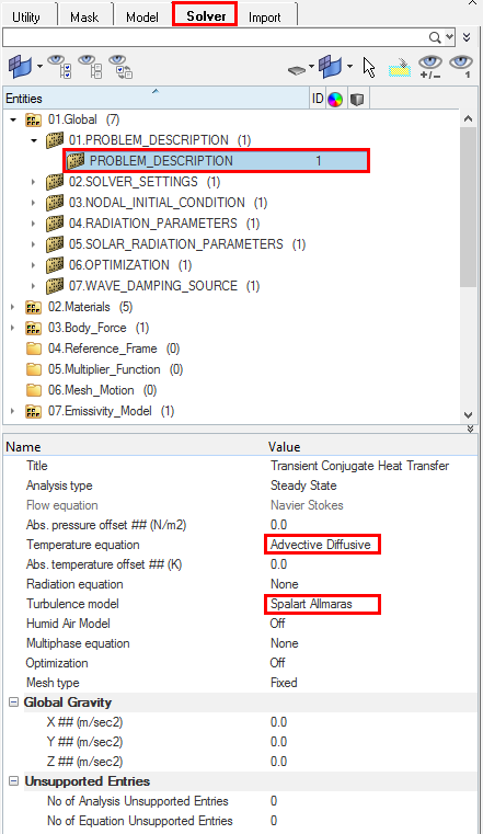
Figure 2.
Set Up Boundary Conditions and Material Model Parameters
In this step, you will start by creating a new material, then you will define the surface boundary conditions for the problem and assign material properties to the fluid and solid volumes.
Create a New Material Model
-
Set the Conductivity to 16.2 W/m-k.
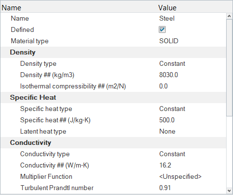
Figure 3.
Set Up Boundary Conditions
-
Click Large_Inlet. In the Entity Editor,
- Change the Type to INFLOW.
- Set the Inflow type to Average velocity.
- Set the Average velocity to 0.4 m/s.
- Set the Temperature to 295.0 K.
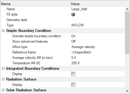
Figure 4. -
Click Outflow. In the Entity Editor, change the Type to
OUTFLOW.
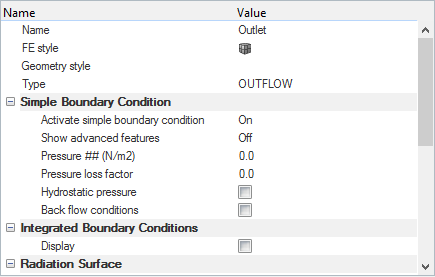
Figure 5. -
Click Symmetry. In the Entity Editor, change the Type to
SYMMETRY.
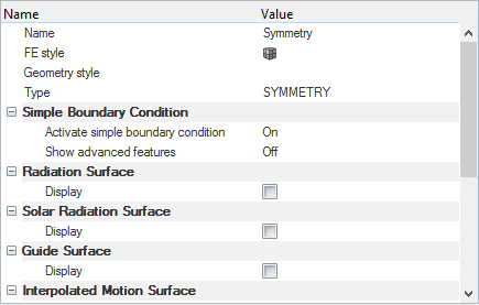
Figure 6. -
Click Pipe_OuterWalls. In the Entity Editor,
- Verify that the Type is set to WALL.
- Set the Convective heat flux coefficient to 100 J/m2-sec-K.
- Enter 302.594 K for the Convective heat flux reference temperature.
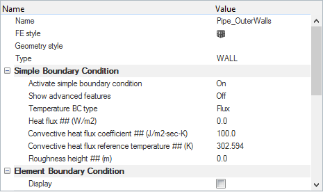
Figure 7. -
Click Pipe_InnerWalls. In the Entity Editor,
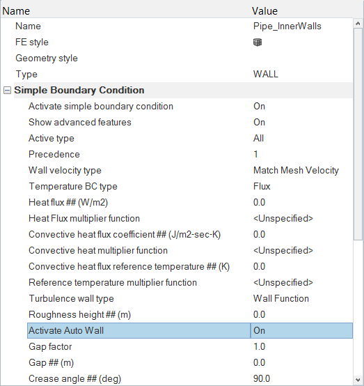
Figure 8. -
Click Pipe_Ends. In the Entity Editor,
- Verify that the Type is set to WALL.
- Change the Temperature BC type to None.
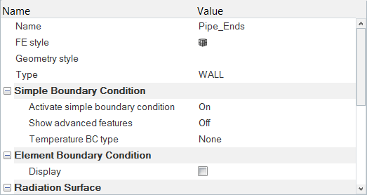
Figure 9. -
Click Fluid. In the Entity Editor,
- Change the Type to FLUID.
- Select Water_HM as the Material.
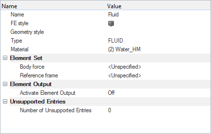
Figure 10. -
Click Solid. In the Entity Editor, and
- Change the Type to SOLID.
- Select Steel as the Material.
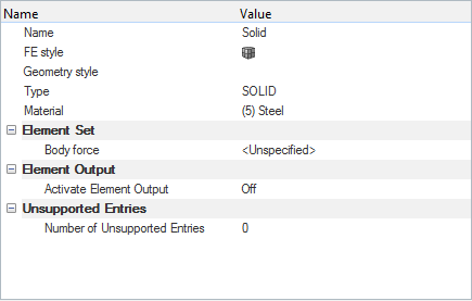
Figure 11.
Compute the Solution
In this step, you will launch AcuSolve directly from HyperMesh and compute the solution.
Run AcuSolve
-
Click
 on the ACU toolbar.
The Solver job Launcher dialog opens.
on the ACU toolbar.
The Solver job Launcher dialog opens. -
Leave the remaining options as
default and click Launch to start the solution
process.
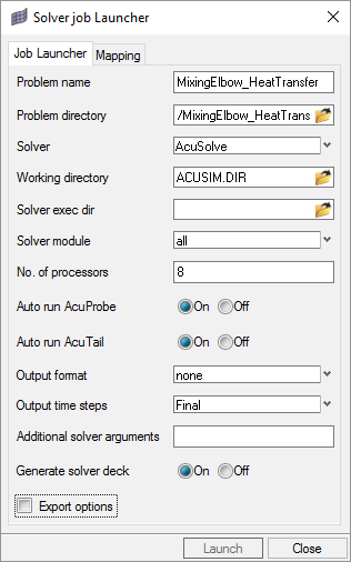
Figure 12.
Post-Process the Results with HyperView
Open HyperView and Load the Model and Results
-
In the Load model and results panel, click
 next
to Load model.
next
to Load model.
Create Contours for Temperature Distribution
-
Click the Isolate Shown icon
 then hold Ctrl and select the
Symmetry and Pipe_Symmetry
components to turn off the display of all components in the graphics window
except the Symmetry and Pipe_Symmetry components.
then hold Ctrl and select the
Symmetry and Pipe_Symmetry
components to turn off the display of all components in the graphics window
except the Symmetry and Pipe_Symmetry components.
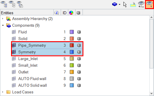
Figure 13. -
Orient the display to the xy-plane by clicking
 on the Standard Views toolbar.
-
Click
 on the Results toolbar to open the Contour panel.
-
In the panel area, under the Display tab, turn off
the Discrete color option.
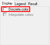
Figure 14. -
Click the Legend tab then
click Edit Legend. In the dialog, change the Numeric
format to Fixed then click
OK.
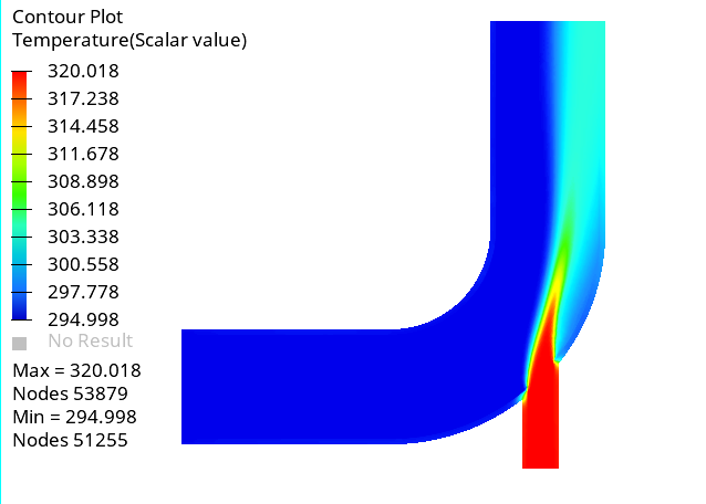
Figure 15.Next, you will display temperature contours on the outlet surface.
-
Click
 on the Standard Views toolbar.
-
In the panel area, click Apply.
The contour plot on the outlet surface is displayed.
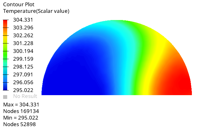
Figure 16.
Summary
In this tutorial, you learned how to set up a conjugate heat transfer CFD simulation using HyperMesh and how to create a new material model. You launched AcuSolve directly from HyperMesh to compute the solution and then post-processed the results using HyperView.