HM-4620: Create Rigid Walls, Model Data, Constraints, Cross Sections, and Output with LS-DYNA
In this tutorial you will: create *PART_INERTIA for the vehicle mass component, velocity on all nodes except barrier nodes with *DEFINE_BOX and *INITIAL_VELOCITY, a contact between the crash boxes, the bumper, and the barrier with *CONTACT_AUTOMATIC_GENERAL, and a stationary rigid wall; use *DATABASE_HISTORY_NODE to specify nodes to be output; use *DATABASE_CROSS_SECTION_PLANE to specify the output of resultant forces; and make nodes a part of the mass rigid body with *CONSTRAINED_EXTRA_NODES.
Overview of *PART_INERTIA, *CONSTRAINED_EXTRA_NODES, *DATABASE_CROSS_SECTION_(Option), and *RIGIDWALL
In this section, you will learn about *PART_INERTIA, *CONSTRAINED_EXTRA_NODES, *DATABASE_CROSS_SECTION_(Option), and *RIGIDWALL.
*PART_INERTIA
The INERTIA option enables inertial properties and initial conditions to be defined rather than calculated from the finite element mesh. This applies to rigid bodies only. When importing a LS-DYNA model into Engineering Solutions, the *PART_INERTIA IRCS parameter value is changed from 0 to 1. The inertia components are changed from global to local axis.
This allows inertia components to be automatically updated when *PART_INERTIA elements are translated or rotated. When selecting *PART_INERTIA elements to translate or rotate, select elements by comp. This selection method ensures the inertia properties are automatically updated.
*CONSTRAINED_EXTRA_NODES
This card defines extra nodes to be part of a rigid body. In Engineering Solutions, it is created from the Solver Browser or Model Browser, Create Cards menu (access from the Tools pull-down menu), or the Quick Access tool (Ctrl + F) when a keyword is entered.
*DATABASE_CROSS_SECTION_(Option)
*DATABASE_CROSS_SECTION_(Option) defines a cross section for resultant forces written to the ASCII SECFORC file. The options are PLANE and SET.
For the PLANE option, a cutting plane must be defined. For best results, the plane should cleanly pass through the middle of the elements, distributing them equally on either side.
The SET option requires the equivalent of the automatically generated input via the cutting plane to be identified manually and defined in sets. All nodes in the cross-section and their related elements contributing to the cross-sectional force resultants should be defined in sets.
*DATABASE_CROSS_SECTION_SET and *DATABASE_CROSS_SECTION_PLANE are created from the Solver Browser or Model Browser, Create Cards menu (access from the Tools pulldown menu), or the Quick Access tool (Ctrl + F) when a keyword is entered.
*RIGIDWALL
A *RIGIDWALL provides a method for treating contact between a rigid surface and nodal points of a deformable body.
In Engineering Solutions, *RIGIDWALL keyword cards are created from the Solver Browser or Model Browser, Create Cards menu (access from the Tools pull-down menu), or the Quick Access tool (Ctrl + F) when a keyword is entered.
Load the LS-DYNA User Profile
In this step, you will load the LS-DYNA user profile in Engineering Solutions.
- Start Engineering Solutions Desktop.
- In the User Profile dialog, set the user profile to LsDyna.
Import the LS-DYNA Model
In this step, you will import the LS-DYNA model file into Engineering Solutions.
Define *PART_INERTIA
In this step, you will define *PART_INERTIA for the vehicle mass component to partially take into account the inertia properties and mass of the missing parts.
-
In the Model Browser, Components folder, click
vehicle mass.
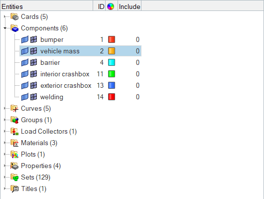
Figure 1.The Entity Editor opens, and displays the component's card data.
Create a *DEFINE_BOX that Contains Non-Barrier Nodes
In this step, you will create a *DEFINE_BOX in Engineering Solutions that contains all nodes except barrier nodes.
-
In the Solver Browser, right-click and select from the context menu.
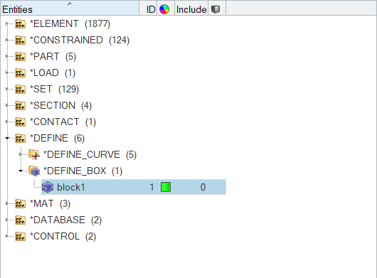
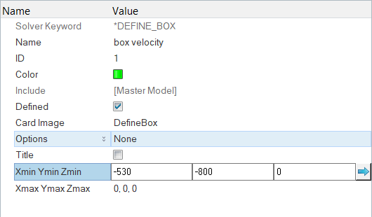
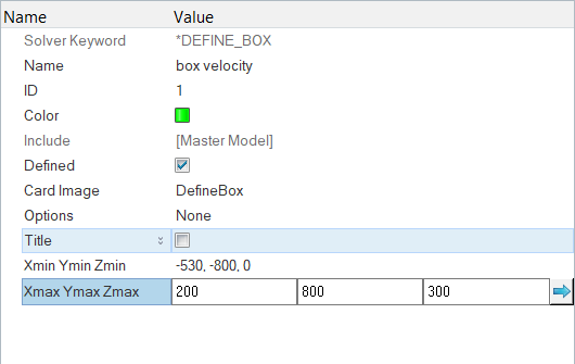
Figure 2.A new block opens in the Entity Editor. - In the Entity Editor, define the block.
Create Initial Velocity
In this tutorial, you will create initial velocity on all nodes except barrier nodes.
-
In the Solver Browser, right-click and select from the context menu.
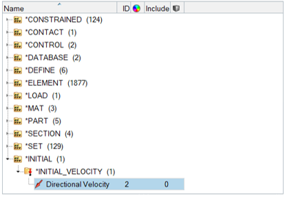
Figure 5.A new load opens in the Entity Editor. -
In the Entity Editor, define the load.
-
Click BOXID, and then click
Block.
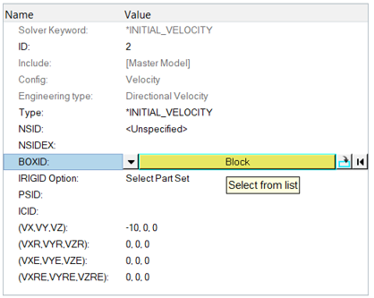
Figure 6. -
In the Select Block dialog, select box
velocity and then click OK.
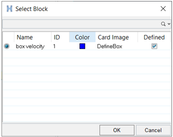
Figure 7.
-
Click BOXID, and then click
Block.
View the Nodes in the Node Entity Set
In this step, you will view the closest nodes which are in the pre-defined node entity set (*SET_NODES_LIST) named Constrain Vehicle using two methods.
-
Method 1
-
In the Solver Browser, SET folder, SET_NODE_LIST
folder, right-click on Constrain Vehicle and
select Review from the context menu.
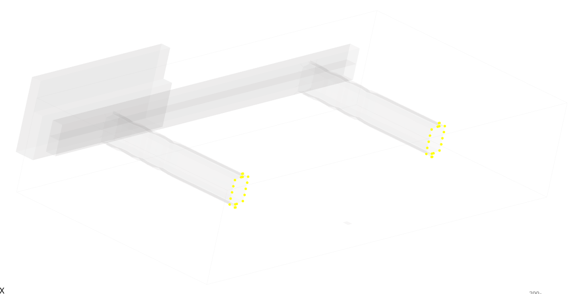
The set's nodes highlight as seen in Figure 8.
Figure 8. -
Right-click on Constrain Vehicle and select
Review from the context menu.
The entities return to their original display color as seen in Figure 9.
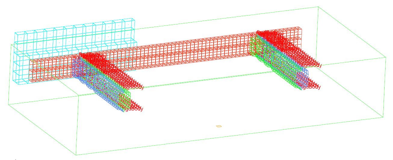
Figure 9.
-
In the Solver Browser, SET folder, SET_NODE_LIST
folder, right-click on Constrain Vehicle and
select Review from the context menu.
- Method 2
Create *CONSTRAINED_EXTRA_NODES_SET
In this step, you will create a *CONSTRAINED_EXTRA_NODES_SET.
-
In the Solver Browser, right-click and select from the context menu.
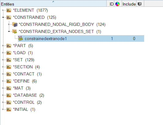
Figure 12.A new constrained extra node opens in the Entity Editor. -
In the Entity Editor, define the constrained extra
node.
-
For PID, click .
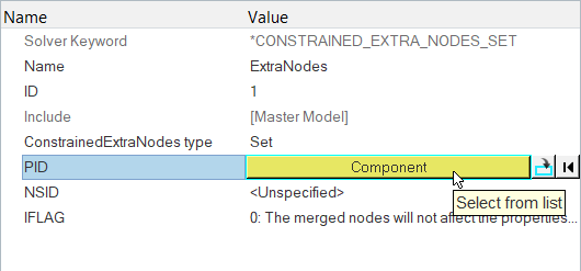
Figure 13. -
In the Select Component dialog, select
vehicle mass and then click
OK.
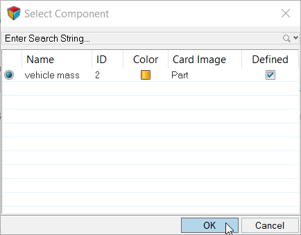
Figure 14.
-
For PID, click .
Define Nodes in the Constrain Vehicle
In this step, you will define the nodes in the Constrain Vehicle set to be a part of the vehicle mass rigid body.
- For NSID, click .
- In the Select Set dialog, select Constrain Vehicle and then click OK.
View Extra Nodes of the Vehicle Mass Rigid Body
In this step, you will view the extra nodes that are a part of the vehicle mass rigid body.
-
Review ExtraNodes by completing one of the following options:
- In the Solver Browser right-click on ExtraNodes and select Review (press Q) from the context menu.
- In the Model Browser right-click on ExtraNodes and select Review (press Q) from the context menu.
The extra nodes temporarily display red, the PID (vehicle mass) displays blue, and all of the other entities temporarily display grey as seen in Figure 15.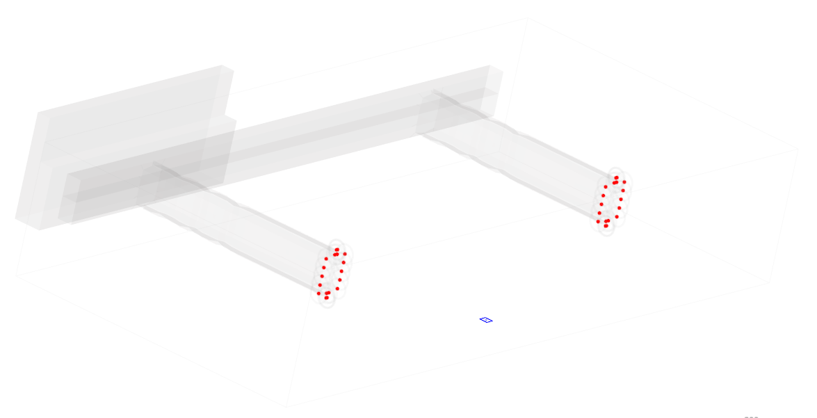
Figure 15.
Create an Entity Set
In this step, you will create an entity set, *SET_PART_LIST, for the vehicle mass component.
-
In the Solver Browser, right-click and select from the context menu.
Tip: You can also create a *SET_PART_LIST from the Model Browser, Create Cards menu (access from the Tools pull-down menu), or the Quick Access tool (Ctrl + F) when a keyword is entered.
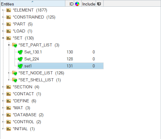
Figure 16.A new set opens in the Entity Editor.
Create a *CONTACT_AUTOMATIC_GENERAL Contact
In this step, you will create a *CONTACT_AUTOMATIC_GENERAL contact.
-
In the Solver Browser, right-click and select from the context menu.
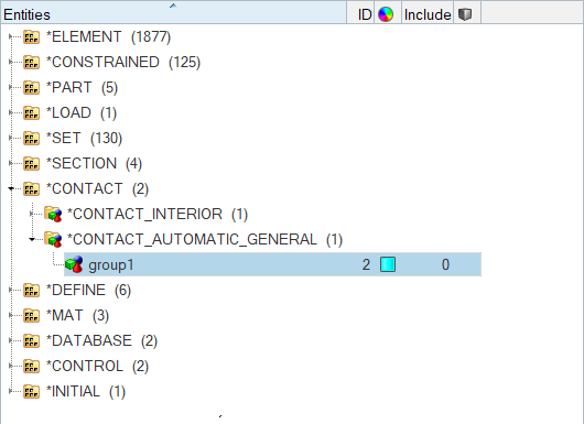
Figure 17.A new group opens in the Entity Editor.
Define Secondary Surface
In this step, you will define the secondary surface with secondary set type 6, part set ID for exempted parts.
-
Select the ExemptSlvPartSet checkbox.
The SSTYPE (secondary surface type) value changes from 2 (part set ID) to 6 (part set ID for exempted parts) as seen in Figure 18.
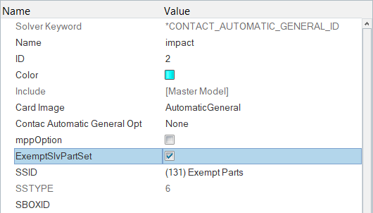
Figure 18.
Create an Entity Set
In this step, you will create an entity set, *SET_PART_LIST, to specify the elements that will contribute to the cross-sectional force results.
-
In the Solver Browser, right-click and select from the context menu.
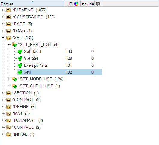
Figure 19.A new group opens in the Entity Editor.
Define a Section
In this step, you will define a section by creating a *DATABASE_CROSS_SECTION_PLANE.
-
In the Solver Browser, right-click and select from the context menu.
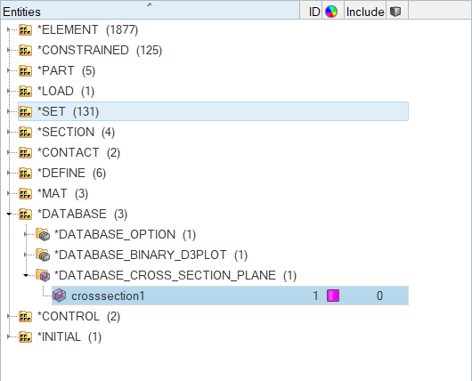
Figure 20.A new group opens in the Entity Editor.
Define the Location and Size of the Section Plane
In this step, you will define the location and size of the section plane.
-
Create a base node.
-
In the z field, enter 100.
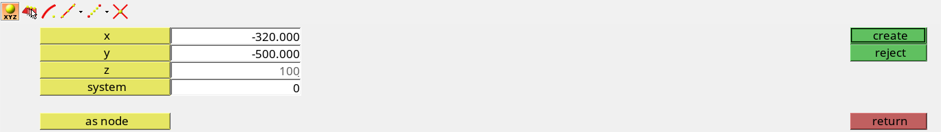
Figure 21. -
Click create.
A new node displays as seen in Figure 22.
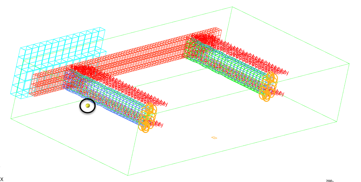
Figure 22.
-
In the z field, enter 100.
-
In the Entity Editor, define the XTAIL, YTAIL, ZTAIL
(base node) for the section.
-
Click XTAIL, YTAIL, ZTAIL (base node), and then
click
 .
.
-
In the graphics area, select the base node you created in step 1 as seen in
Figure 23.
Note: If the base node is not visible, click
 on the Visualization toolbar to display
elements as a wireframe (skin only).
on the Visualization toolbar to display
elements as a wireframe (skin only).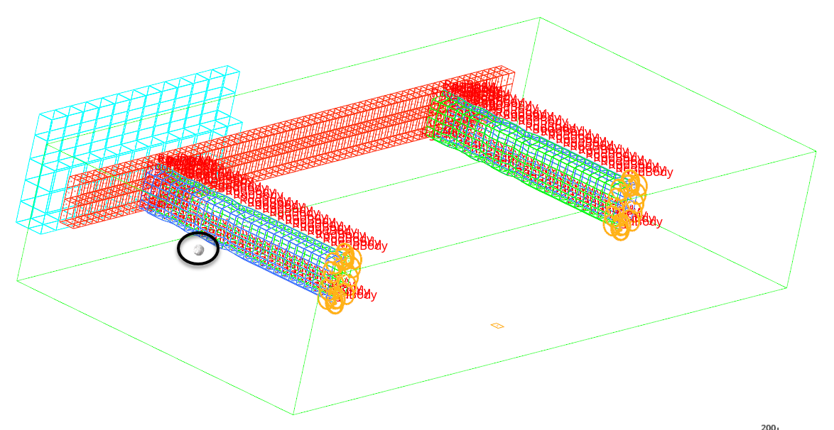
Figure 23. -
Click proceed.
The Entity Editor displays the coordinates of the base node in the XTAIL, YTAIL, ZTAIL field as seen in Figure 24.
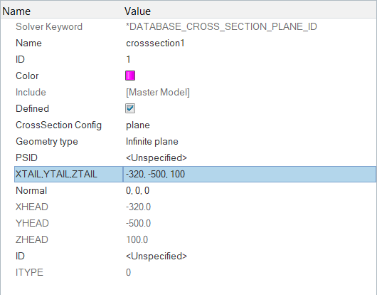
Figure 24.
-
Click XTAIL, YTAIL, ZTAIL (base node), and then
click
-
Define the normal vector.
-
Click Normal, and then click .
- In the panel area, set the orientation selector to x-axis.
- Click proceed.
-
Click Normal, and then click
-
Define the edge vector.
-
Click Edge, and then click .
-
Click Edge, and then click
-
For LENM (length of edge b, in the M direction), enter
200.
Tip: If you know the coordinates of the base node, edge, and normal, you can manually enter them in the Entity Editor.
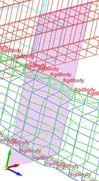
Figure 25.
Specify the Parts Secondary to the Cross Section
In this step, you will specify the parts secondary to the cross section.
- For PSID, click .
- In the Select Set dialog, select CrossSectionPlane-Parts and then click OK.
View the Entities Secondary to the Rigid Wall
In this step, you will view the entities secondary to the rigid wall.
-
In the Solver Browser, right-click on
CrossSection_Plane and select
Review from the context menu.
The secondary entities and rigid wall highlight and all of the other entities temporarily display grey as seen in Figure 26.
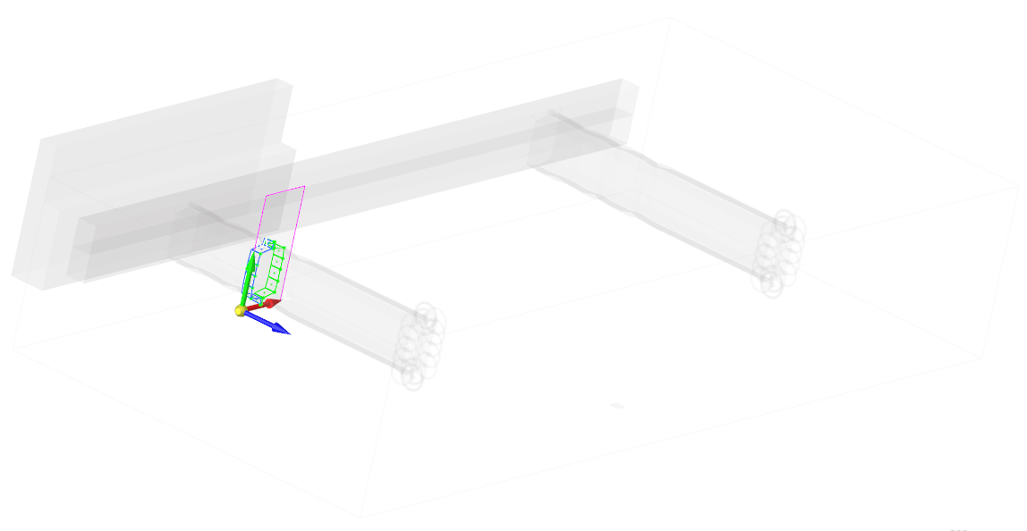
Figure 26.
Create a *DEFINE_BOX that Contains Barrier and Bumper Nodes
In this step, you will create a *DEFINE_BOX containing the nodes making up the barrier and the left side of the bumper.
-
In the Solver Browser, right-click and select from the context menu.
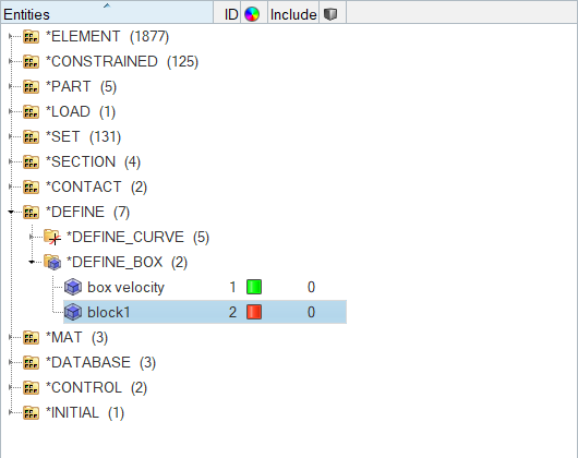
Figure 27.A new block opens in the Entity Editor. -
In the Entity Editor, define the block.
-
For Xmax Ymax Zmax, enter -460,
0, 400.
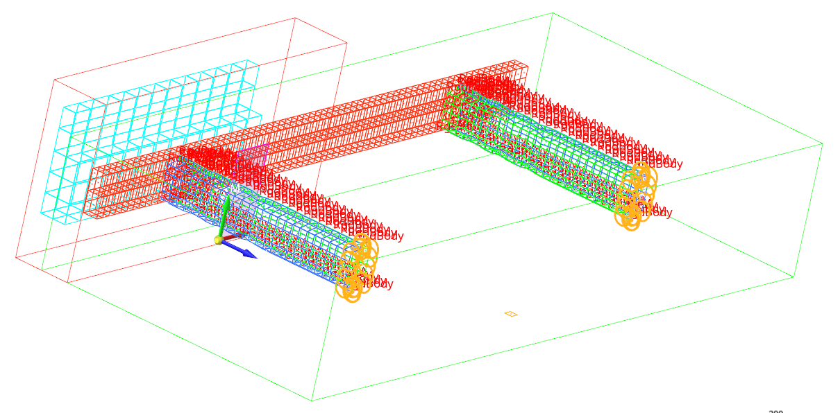
Figure 28.
-
For Xmax Ymax Zmax, enter -460,
0, 400.
Create a *RIGIDWALL_PLANAR_FINITE
In this step, you will define a Engineering Solutions group by creating *RIGIDWALL_PLANAR_FINITE.
-
In the Solver Browser, right-click and select from the context menu.
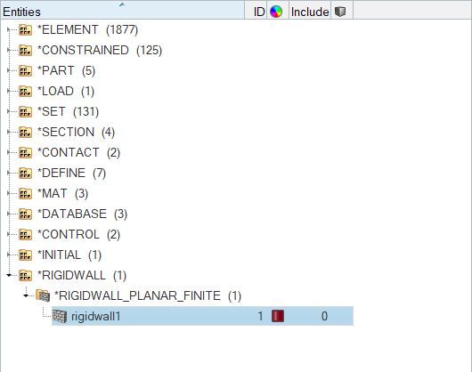
Figure 29.A new rigid wall opens in the Entity Editor.
Define the Location and Size of the Rigid Wall
In this step, you will create a node from the create nodes panel and then select it for the base node.
-
Create a base node.
-
Click
 to open
the XYZ subpanel.
to open
the XYZ subpanel.
-
Click create.
Tip: If the base node is not visible, click on the Visualization toolbar to display elements as a wireframe
(skin only).
-
Click
-
For XT, YT, and ZT enter -600,
-750, and 90 as seen in Figure 30.
Note: You can also select the node created in step 1 for the rigid wall base.
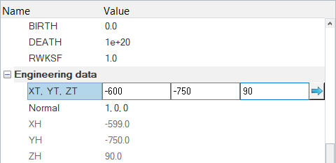
Figure 30. -
Define the normal vector.
-
Click Normal, and then click .
- In the panel area, set the orientation selector to x-axis.
- Click proceed.
-
Click Normal, and then click
-
Define the edge vector.
-
Click Edge, and then click .
- In the panel area, set the orientation selector to y-axis.
- Click proceed.
-
Click Edge, and then click
-
For Length LENM, enter 250.
Note: The input values for LENL and LENM are the length of the edges a and b in the L and M directions, respectively. These values define the extent of the rigid wall.
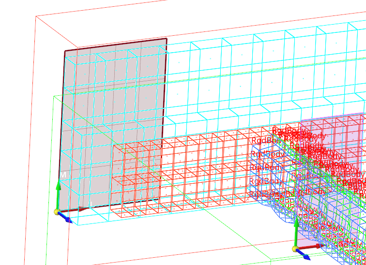
Figure 31.
Specify Nodes as Secondary to the Rigid Wall
In this step, you will use the Entity Editor for the rigid wall to specify the nodes in the *DEFINE_BOX half model as secondary to the rigid wall.
- Click .
- In the Select Block dialog, select half model and then click OK.
- For FRIC (Interface friction), enter 1.0.
Specify Nodes to be Output
In this step, you will specify some nodes to be output to the ASCII NODOUT file with *DATABASE_HISTORY_NODE.
-
In the Solver Browser, right-click and select from the context menu.
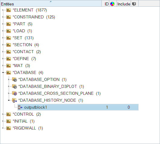
Figure 32.A new output block opens in the Entity Editor. -
In the Entity Editor, define the output block.
-
In the graphics area, select a few nodes of interest as seen in Figure 33.
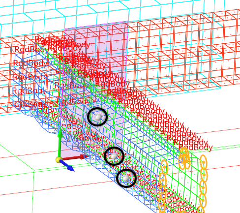
Figure 33.
-
In the graphics area, select a few nodes of interest as seen in Figure 33.
Export the Model
In this step, you will export the model to an LS-DYNA 971_R# formatted input file.
Submit the Input File
In this step, you will submit the LS-DYNA input file to the LS-DYNA 970 solver.
- From the Start Menu, open the LS-DYNA Manager program.
- From the solvers menu, select Start LS-DYNA analysis.
- Load the bumper_complete.key file.
- Start the analysis by clicking OK.
View the results in HyperView
In this step, you will view the results in HyperView.