CFD-1600: Map CFD Results
This exercise will cover how to take results from a CFD analysis and apply them to a new model for heat transfer or structural analysis. Using the linear interpolation tools within Engineering Solutions, results from a CFD analysis can be transferred to be loads in an analysis to be run in OptiStruct or any other supported solver.
Typically, scalar results such as temperatures or pressures are mapped. Results must be in a Tecplot file (*.tpl or *.dat). This exercise will demonstrate how Engineering Solutions has a very easy and straightforward way to transfer loads from CFD to a heat transfer of structural analysis.
The model file used in this exercise can be found in the es.zip file. Copy the file(s) from this directory to your working directory.
Load the CFD User Profile
-
From the menu bar, click or click the Load User Profile icon,
 , on
the Standard toolbar.
, on
the Standard toolbar.
- Click .
- Click OK.
Open the Model File
-
On the Standard toolbar, click the Open Model
 icon.
icon.
-
Use the Model Browser to turn off the display of the
component cube.
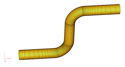
Figure 1.
Load and Process Tecplot File
Create a Load Collector for the Pressure Loads
-
For Name enter pressure.
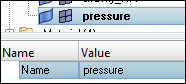
Figure 2.
Map the Load Pressure to the New File
-
Next to nodes on face, click nodes and then select three
nodes that define an element.
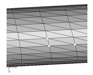
Figure 3.
Turn Off the Display of the Load Collector and Show Pressure Loads As a Contour Plot
-
To turn off the display of the load collector pressure, click the
 icon to the left of pressure.
The icon will be grayed out and the pressure loads will no longer be displayed.
icon to the left of pressure.
The icon will be grayed out and the pressure loads will no longer be displayed. -
Click contour.
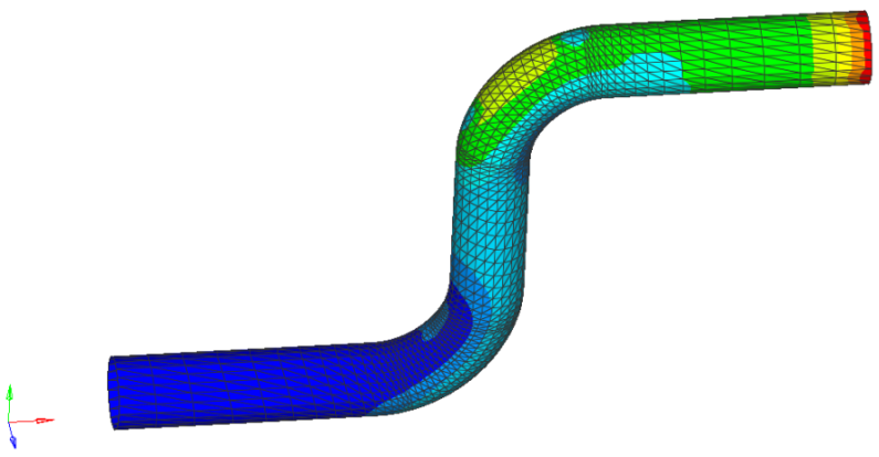
Figure 4.This simply displays the pressure load as a contour for an easier way to view the load. Now that the pressure load has been applied, an additional analysis can be set up and run.