Element Biasing
The automeshing process enables you to bias the placement of nodes so that their intervals are not uniform in size.
You can designate that the smaller intervals go near the start of the edge, near the end of the edge, near both ends with larger intervals in the middle, or near the middle of the edge.
Within the automesher, you may want to use biasing to improve element quality when transitioning from smaller to larger element sizes. When you use the Drag and Solid Offset panels, you can use biasing to cluster several layers of elements near the surface of a solid. In Linear Solids, the mesh at one end could be scaled several times larger than at the other end. Element biasing allows you to moderate the changes in aspect ratio from the start to the end.
Linear Biasing
In linear biasing, the biasing intensity corresponds to the positive slope of a straight line over the interval [0,1] of the Real Line. This interval is uniformly divided into as many subintervals as specified by the element density and they are mapped along the edge so that the length of the image interval is proportional to the height of the line over the midpoint of the source interval. Each image interval corresponds to the side of an element.
Specifically, let n be the element density and let 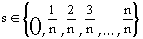 .
.
We want a node placement function x(s) taking values in [0,1] with x(0) = 0 and x(1) = 1. If m is the slope of the line, and b is its y-intercept, then:
![]() .
.
Using x(0) = 0, and x(1) = 1, we find: ![]() so,
so,
![]() .
.
For this, m is the absolute value of the biasing intensity. If the biasing intensity is negative, the nodes are placed according to 1 - x(s). Thus, a positive biasing intensity puts small elements at the start of the interval.
We can use b to scale the behavior of the function so that convenient values are in the range [0,20]. The value used is b = 1.5.
Exponential Biasing
In exponential biasing, the sizes of the intervals grow geometrically, progressing along the edge, with each successive interval being a constant factor larger than the previous. That factor is 1.0 plus 1/10 of the absolute value of the biasing intensity. This formula was chosen so that an intensity of zero will still represent no biasing, and convenient values will fall in the range [0,20]. Negative biasing intensities just reverse the edge, placing the smaller elements at the end instead of the beginning.
Specifically, let n be the element density and let ![]() .
.
We want a node placement function x(s) taking values in [0,1] with x(0) = 0 and x(1) =1.
Let ![]() be the geometric
growth factor.
be the geometric
growth factor.
We need a function ![]() so that:
so that: 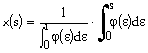
Let ![]() then:
then:
![]() which gives the
proper interval lengths,
which gives the
proper interval lengths,
then x(s) scales them to the range of [0,1]. Thus, ![]() .
.
Bellcurve Biasing
In bellcurve biasing, nodes are distributed long the edge in a pattern that is symmetric across the midpoint of the edge. If the biasing intensity is positive, the smaller intervals are placed at the beginning and end of the edge, and if it is negative, they are placed at the middle of the edge.
Specifically, let n be the element density and ![]() .
.
We need ![]() so that
so that
takes values in [0,1] with x(0) = 0, x(1) = 1, and has the behavior noted above. If we use:
![]() for positive biasing
intensity r, then x(s) becomes:
for positive biasing
intensity r, then x(s) becomes:
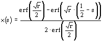 where erf() is the
statistical error function,
where erf() is the
statistical error function,
 .
.