MV-1028: Model a Point-to-Deformable-Surface Higher-Pair Constraint
In this tutorial, you will learn how to model a PTdSF (point-to-deformable-surface) joint.
Create Points
In this step, you will create points for the PTdSF model.
-
Open the Add Point or PointPair dialog in one of the
following ways:
- From the Project Browser right-click on Model and select .
- On the Model-Reference toolbar, right-click the
 (Point) icon.
Create Bodies
In this step you will create the membrane and ball bodies for the PTdSF model.
-
Open the Add Body or BodyPair dialog in one of the
following ways:
- From the Project Browser right-click on Model and select .
- On the Model-Reference toolbar, right-click on the
 (Body) icon.
-
Click the
 (Graphic file browser) icon and select
membrane.h3d from the <working
directory>.
(Graphic file browser) icon and select
membrane.h3d from the <working
directory>.
-
Double click
 .
.
Create Markers and a Deformable Surface
In this step you will define markers for the membrane.
-
On the general toolbar, click .
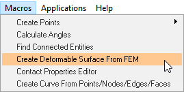
Figure 1. -
In the panel, double-click
 .
.
-
Double-click on
 .
.
-
Next to Select the FEM file, click the (file
browser) icon.
-
Select the membrane.fem file from your working directory
and click OK.
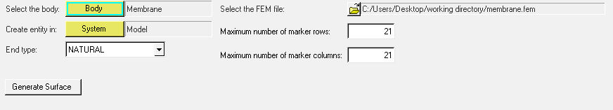
Figure 2.
Create Joints
In this step you will define four fixed joints between the membrane and the ground.
-
Open the Add Joint or JointPair dialog in one of the
following ways:
- From the Project Browser, right-click on Model and select .
- On the Model-Constraint toolbar, click the
 (Joints) icon.
-
In the Joint panel, configure the Connectivity tab.
-
Double-click
 .
.
- In the dialog, select Membrane and click OK.
-
Double-click
 .
.
- In the dialog, select Ground Body and click OK.
-
Double-click .
- In the dialog, select PointMembInterface39 and click OK.
-
Double-click
Create the PTdSF Joint
In this step, you will define the PTdSF (point-to-deformable-surface) joint as an advanced joint.
-
Open the Add AdvJoint dialog by doing one of the
following:
- From the Project Browser, right-click on Model and select .
- On the Model-Constraint toolbar, click the
 (Advanced Joint)
icon.
(Advanced Joint)
icon.
- In the dialog, for Label enter AdvancedJoint 0. Accept the default variable name.
- In the Type drop-down menu, click PointToDeformableSurface Joint.
- Click OK.
-
In the panel, configure the Connectivity tab.
-
Double-click and select
Ball.
- Click OK.
-
For , choose BallCM and
click OK.
-
For
 , choose DeformableSurface
1 and click OK.
, choose DeformableSurface
1 and click OK.
-
Double-click
Create Graphics
In this step, you will create a graphic for the ball.
-
Open the Add Graphics or GraphicPair dialog in one of the
following ways:
- From the Project Browser, right-click on Model and select .
- On the Model-Reference toolbar, click the
 (Graphics) icon.
- In the dialog, for Label enter Ball.
- In the Type drop-down menu, choose Sphere. Then click OK.
-
In the Connectivity tab, double-click .
- In the dialog, select Ball and click OK.
-
Double-click on .
- In the dialog, select BallCM and click OK.
- In the Properties tab, under Radius enter 1.0.
- In the Visualization tab, choose a color for the graphic.
Find Nodes
In this step, you will return to the Bodies Panel and find the Nodes on the membrane.
-
On the reference toolbar, click the (Bodies) icon.
-
Close the dialog.
Your model should resemble the example shown in Figure 3.
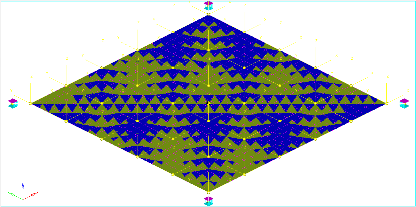
Figure 3.
Run the Model
In this step, you will run the model with a PTdSF constraint.
-
On the toolbar, click
 (Run).
-
In the Run panel, specify the values shown in Figure 4.
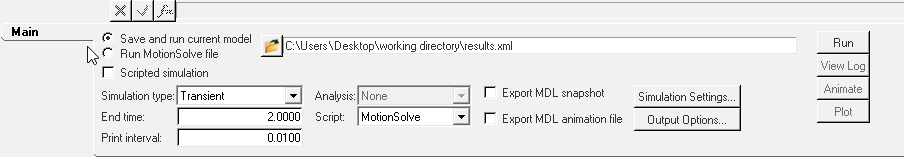
Figure 4. -
Click the
 (browser icon) and specify
result.xml as the file name.
(browser icon) and specify
result.xml as the file name.
-
Specify the Maximum step size as 0.001 (as the solution
is not converged for the default step size of 0.01).
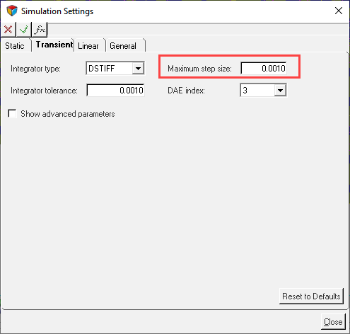
Figure 5. -
Click the
 (Check Model) button to check the model for
errors.
(Check Model) button to check the model for
errors.
View the Results
In this step, you will view the animation and plot the Z position of the center of mass of the ball.
-
Once the solver has finished, the Animate button will be active. Click on
Animate.
Click the
 (Start/Pause Animation) button
to view the animation.
(Start/Pause Animation) button
to view the animation.One would also like to inspect the displacement profile of the membrane and the ball. For this, we will plot the Z position of the center of mass of the ball.
-
Click on the
 (Add Page) icon.
-
In the Select application drop-down menu, change the client from MotionSolve
 to HyperGraph 2D
 .
.
-
On the Curves toolbar, click
 (Build Plots).
-
Click the (file browser) and open the
results.abf file.
-
Configure the Plots panel as show in Figure 6.
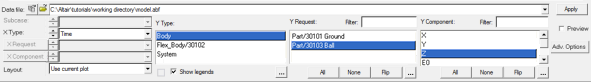
Figure 6. -
Click Apply.
The profile for the Z-displacement should look like the example given in Figure 7.
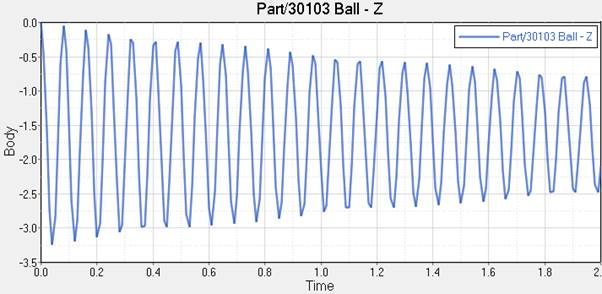
Figure 7.