MV-7002: Co-simulation with Simulink
In this tutorial, you will learn how to use the MotionSolve-Simulink co-simulation interface, driving the model from Simulink via an S-Function. MotionSolve co-simulates with Simulink using the Inter Process Communication (IPC) approach.
In IPC co-simulation, the two solvers are run on two separate processes with data being exchanged through sockets.
Software and Hardware Requirements
- MotionSolve
- MATLAB/Simulink (MATLAB Version R2015a), Simulink Version 8.5) (or newer)
- PC with 64-bit CPU, running Windows 7/10 or higher
- Linux RHEL 6.6 or CentOS 7.2Note: MATLAB R2019a and higher require Windows 10 and RHEL 7.8.
Inverted Pendulum Controller
Consider an inverted pendulum, mounted on a cart. The pendulum is constrained at its base to the cart by a revolute joint. The cart is free to translate along the X direction only. The pendulum is given an initial rotational velocity causing it to rotate about the base.

Figure 1. Inverted Pendulum Model Setup
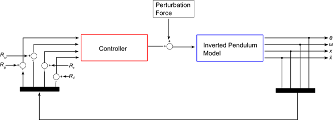
Figure 2. Block Diagram Representation of the Controller
- is the angular displacement of the pendulum from its model configuration
- is the angular velocity of the pendulum about its center of gravity as measured in the ground frame of reference
- is the translational displacement of the cart measured from its model configuration in the ground frame of reference
- is the translational velocity of the cart measured in the ground frame of reference
- is a reference signal for the pendulum's angular displacement
- is a reference signal for the pendulum's angular velocity
- is a reference signal for the cart's translational displacement
- is a reference signal for the cart's translational velocity
A disturbance is added to the computed control force to assess the system response. The controller force acts on the cart body to control the displacement and velocity profiles of the cart mass.
- Solve the baseline model in MotionSolve only (that is, without co-simulation) by using the inverted pendulum model with a continuous controller modeled by a Force_Vector_OneBody element. You can use these results to compare to an equivalent co-simulation in the next steps.
- Review a modified MotionSolve inverted pendulum model that mainly adds the Control_PlantInput and Control_PlantOutput entities that allow this model to act as a plant for Simulink co-simulation.
- Review the controller in Simulink.
- Perform a co-simulation and compare the results between the standalone MotionSolve model and the co-simulation model.
Before you begin, copy all the files in the <installation_directory>\tutorials\mv_hv_hg\mbd_modeling\motionsolve\cosimulation folder to your working directory (referenced as <working directory> in the tutorial). Here, <altair> is the full path to the product installation.
Run the Baseline MotionSolve Model
In this step, use a single body vector force (Force_Vector_OneBody) to model the control force in MotionSolve. The force on the cart is calculated as:
, where
is the disturbance force,
is the control force,
are gains applied to each of the error signals
is the error (difference between reference and actual values) on the input signals.
The angular displacement and velocity of the pendulum are obtained by using the AY() and WY() expressions respectively. The translational displacement and velocity of the cart are obtained similarly, by using the DX() and VX() expressions.
-
From the Start menu, select . Open the model
InvertedPendulum_NoCosimulation.mdl from your <working directory>.
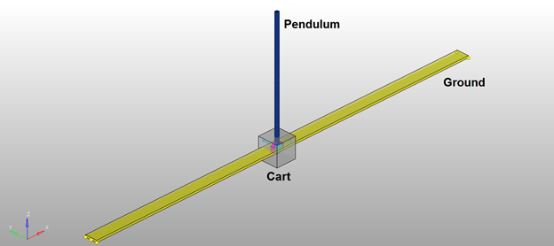
Figure 3. The MotionSolve Model of the Inverted PendulumThe MotionSolve model consists of the following components:
Component Name Component Type Description Slider cart Rigid body Cart body Pendulum Rigid body Pendulum body Slider Trans Joint Translational joint Translational joint between the cart body and the ground Pendulum Rev Joint Revolute joint Revolute joint between the pendulum body and the cart body Control Force Vector force The control force applied to the cart body Output control force Output request Use this request to plot the control force Output slider displacement Output request Use this request to plot the cart's displacement Output slider velocity Output request Use this request to plot the cart's velocity Output pendulum displacement Output request Use this request to plot the pendulum's displacement Output pendulum velocity Output request Use this request to plot the pendulum's velocity Pendulum Rotation Angle Solver variable This variable stores the rotational displacement of the pendulum via the expression AY() Pendulum Angular Velocity Solver variable This variable stores the rotational velocity of the pendulum via the expressionVY() Slider Displacement Solver variable This variable stores the translational displacement of the cart via the expression DX() Slider Velocity Solver variable This variable stores the translational velocity of the cart via the expression VX()
Define the Plant in the Control Scheme
A MotionSolve model needs a mechanism to specify the input and output connections to the Simulink model. The MotionSolve model (XML) used above is modified to include the Control_PlantInput and Control_PlantOutput model elements and provide these connections. In this tutorial, this has already been done for you, and you can see this by opening the model InvertedPendulum_Cosimulation.mdl from your <working directory>.
This model contains two additional modeling components:
| Component Name | Component Type | Description |
|---|---|---|
| Plant Input Simulink | Plant input | This Control_PlantInput element is used to define the inputs to the MotionSolve model |
| Plant Output Simulink | Plant output | This Control_PlantOutput element is used to define the outputs from the MotionSolve model |
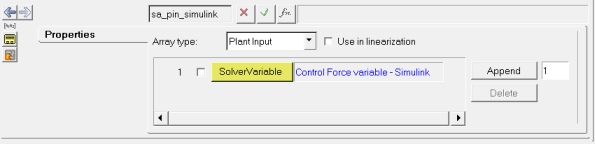
Figure 4. The Definition of the Input Channel to MotionSolve
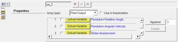
Figure 5. The Definition of the Output Channels from MotionSolve
The inputs specified using the Control_PlantInput and Control_PlantOutput elements can be accessed using the PINVAL() and POUVAL() functions, respectively. Since the Control_PlantInput and Control_PlantOutput list the IDs of solver variables, these input and output variables may also be accessed using the VARVAL() function. For more details, please refer to the MotionSolve User's Guide.
This model has the following connections:
- Plant Input: A single control force that will be applied to the cart.
- Plant Output: The pendulum's angular displacement and angular velocity; the cart's translational displacement and velocity.
Set Up Environment Variables
- Control panel (Windows)
- In the shell/command window that calls MATLAB (with the set command on Windows, or the export command on Linux)
- Within MATLAB, via the
setenv() command
An example of the usage of these commands is listed below:
Environment variable Value Windows shell Linux shell MATLAB shell PATH \mypath set PATH=\mypath setenv PATH \mypath setenv('PATH','\mypath')
Set Up the Co-simulation
The core feature in Simulink that creates the co-simulation is an S-Function (System Function) block in Simulink. This block requires an S-Function library (a dynamically loaded library) to define its behavior. MotionSolve provides this library, but the S-Function needs to be able to find it. To help MATLAB/Simulink find the S-Function, you need to add the location of the S-Function to the list of paths that MATLAB/Simulink uses in order to search for libraries.
The S-Function library for co-simulation with MotionSolve is called
mscosimipc – for Inter Process Communication (IPC) using TCP/IP
sockets for communication. This file is installed under
<altair>\hwsolvers\motionsolve\bin\<platform>.
The location of this file needs to be added to the search path of MATLAB for the S-Function to use
mscosimipc.
This can be done in one of the following ways:
-
Use the menu options.
-
From the MATLAB menu, select .
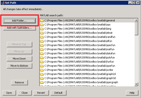
Figure 6. Add path through the MATLAB GUI
-
From the MATLAB menu, select .
-
Use MATLAB commands.
View the Controller Modeled in Simulink
-
Click Open.
You will see the control system that will be used in the co-simulation.
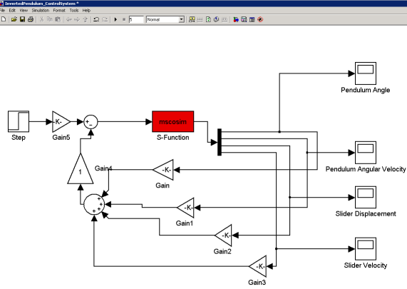
Figure 7. The Control System in MATLAB
Repeat the Co-simulation
-
Check the .log file to make sure no errors or warnings
were issued by MotionSolve.
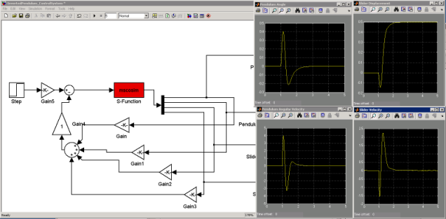
Figure 8.
Compare the MotionSolve-only Results to the Co-simulation Results
-
Click Build Plots
 .
.
-
In the Page Controls toolbar, create two vertical plot windows.
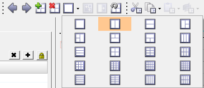
Figure 9. Create Two Plot Windows -
Select Marker Displacement for Y-Type,
REQ/70000004 Output slider displacement (on Slider
cart) for Y Request, and DX for Y
Component to plot the cart's translational displacement:
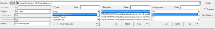
Figure 10. Plot the Cart's Displacement -
Select Marker Force for Y-Type, REQ/70000002
Output control force- (on Slider cart) for Y Request, and
FX for Y Component to plot the X component of the
control force:
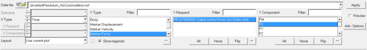
Figure 11. Plot the Control Force on the Cart -
Select Marker Force for Y-Type, REQ/70000002
Output control force- (on Slider cart) for Y Request, and
FX for Y Component to overlay the plot in the right
window.
Both the signals match as shown below.

Figure 12. Comparison of the Cart Displacement and Cart Control Force Between the Two ModelsThe blue curves represent results from the MotionSolve-only model and the red curves represent results from the co-simulation.