ACU-T: 7000 Parametric Optimization with AcuSolve
This tutorial provides instructions for setting up, solving, and viewing results for a parametric optimization problem in AcuSolve. The parametric studies enable you to specify one or more conditions that may vary, such as a sweep over a range of inlet mass flow boundary conditions. The range and frequency of the parameter controlling the mass flow is selected either by simply specifying the desired values or having the program compute suitable values automatically. Several parameters can be used in parametric studies, for instance, controlling the inlet mass flow, the impeller rotational speed, and blade angles of a fan problem. The model used for this tutorial consists of a sphere immersed in a fluid flow. The surface of the sphere is kept hot from an internal heat source. The fluid flow removes the heat from the sphere surface, thus causing the temperature of the fluid to rise. The simulation is run with various values of temperature at the fluid inlet to determine the conditions which result in the outlet temperature closest to a desired value.
- Setting up a parametric optimization problem in AcuSolve
- Post-processing a parametric optimization problem
In this tutorial, you will:
- Analyze the problem
- Import the HyperMesh model database
- Set general simulation parameters and solver settings
- Set material model parameters and nodal initial conditions
- Set up the optimization study parameters
- Assign surface boundary conditions and material properties
- Run AcuSolve
- Monitor the solution with AcuProbe
Prerequisites
Prior to starting this tutorial, you should have already run through the introductory HyperWorks tutorial, ACU-T: 1000 HyperWorks UI Introduction, and have a basic understanding of HyperMesh and AcuSolve. To run this simulation, you will need access to a licensed version of HyperMesh and AcuSolve.
Prior to running through this tutorial, copy HyperMesh_tutorial_inputs.zip from <Altair_installation_directory>\hwcfdsolvers\acusolve\win64\model_files\tutorials\AcuSolve to a local directory. Extract ACU-T7000_ParametricOptimization.hm from HyperMesh_tutorial_inputs.zip.
Since the HyperMesh database (.hm file) contains meshed geometry, this tutorial does not include steps related to geometry import and mesh generation.
Analyze the Problem

Figure 1.
The inlet temperature here is what is known as the “design variable” for the problem. A target value for outlet temperature is specified, and the desired inlet temperature is the value at which the outlet temperature is closest to the target outlet temperature. The difference between the target outlet temperature and the actual outlet temperature is what is known as the “response variable” for the problem. Since the objective of the problem is to minimize the difference between the outlet temperature and the target outlet temperature, this problem is a “minimization” problem.
Optimization
Optimization, in simple terms, is the process of selecting a best input from a set of available alternatives. Almost all engineering problems today are aimed at optimizing something. Airfoil designers are always trying to come up with new airfoil designs with better lift and low drag. Heat exchanger component designers want to maximize the surface heat flux while also minimizing the pressure drop through the exchanger.
AcuSolve offers you two options to setting up an optimization study: design optimization and parametric studies. Design optimization enables you to optimize an objective function subject to certain constraints and satisfaction of flow equations.
Parametric studies enables you to specify one or more conditions that may vary, such as a sweep over a range of inlet mass flow boundary conditions. In parametric studies, these control parameters vary according to a specified pattern. For example, the range and frequency of the parameter controlling the mass flow is selected either by simply specifying the desired values or having the program computing suitable values automatically. Several parameters can be used in parametric studies, for instance, controlling the inlet mass flow, the impeller rotational speed, and blade angles of a fan problem. Perhaps you want to evaluate the pressure rise and torque of the fan; these outputs are called "response variables". The parameters controlling the run conditions are called "variables" or "design variables". The nomenclature is similar to the optimization problems.
- the geometry is allowed to change (geometric design and shape optimization) and/or
- internal parameters, such as the inlet flow rate or viscosity, are allowed to change (design of experiments and quantified optimization).
A minimization problem where a local minimum is sought can be stated as:
Minimize, objective(U,Y)
subject to constraints(U,Y)
Here, U is the flow solution variables and Y is a vector of control parameters, called Design Variables (DVs), that determines the shape of an object or a flow parameter. The objective(s) and constraint(s) are specified by you. A maximization problem is the same as above, but Minimize is replaced with Maximize.
Optimization Solution Sequence
The design optimization may be considered as a sequence of cases, where each case first runs the optimizer and updates the design variables and then solves the flow equations for a number of time steps until convergence. Sample data is gathered at the end of each time step.
- Constructing the response surface from the set of samples.
- Running the optimizer on the response surface.
- Updating the design variables.

Figure 2.
Open the HyperMesh Model Database
-
Click the Open Model icon
 located on the standard toolbar.
The Open Model dialog opens.
located on the standard toolbar.
The Open Model dialog opens.
Set the Global Simulation Parameters
Set the Analysis Parameters
In next steps, you will set parameters that apply globally to the simulation.
-
Set Optimization to On.
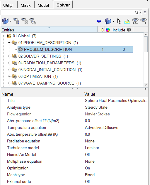
Figure 3.
Specify the Solver Settings
-
Check that the Flow, Temperature, and Design Optimization flags are set to On
and the Temperature flow flag is set to Off.
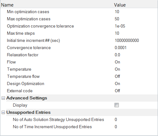
Figure 4.
Set Material Model Parameters
In the next steps, you will create a new custom material and assign relevant material properties to it.
-
Set the Conductivity value to 1.0 W/m-K.
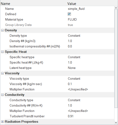
Figure 5.
Set Up the Optimization Parameters
Define the Design Variable
-
Enter 1.0 in row 1, 0.9 in row 2,
and 0.8 in row 3 then click
Close.
The Supervised Training parameter is used to enforce AcuSolve to use the listed design variable values for as many cases as there are values in the list. After the list is exhausted, optimization control takes over. It is advisable to provide at least three values for Supervised Training as it helps the solver develop a pattern, streamlining the process of selecting the values for design variable for succeeding runs.
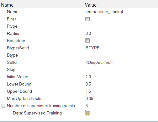
Figure 6.
Create a Multiplier Function for the Design Variable
In AcuSolve, multiplier functions are used to scale values of certain parameters at runtime. For example, viscosity of a fluid may vary with temperature. Or inflow rate or temperature may vary over time.
Multiplier functions can also be used to scale the values of the design variables between cases. In quantity optimization, the design variables are linked with the desired quantities in AcuSolve through multiplier functions.
-
Click in the value field next to Design Variable, click the
Designvar collector, select
temperature_control from the appearing dialog, then
click OK.
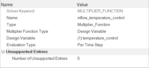
Figure 7.
Define Response Variables
Response variables are the building blocks for deriving objective functions and constraints. Examples include: drag, lift, force in an arbitrary direction, total volume, pressure drop, total pressure, uniformity index on temperature, max speed, etc. In other words, response variables are functions of the flow solution (via output mechanism), the design variables, and/or other response variables.
The most basic response variables are functions of the flow solution, extracted from the SURFACE_OUTPUT and ELEMENT_OUTPUT. More complex response variables can be derived from these basic response variables using expressions. An example of this is demonstrated in the following steps.
-
Click on temperature. In the entity editor,
- Change the Response type to Surface Output.
- Click in the value field next to Surface Elements, click the Component collector, select Outflow from the appearing dialog, and click OK.
- Set the Output variable to Temperature.
This response variable will extract the surface integrated value of the temperature variable from the outflow surface.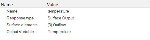
Figure 8.
Define the Objectives
It was mentioned earlier that the response variables are the building blocks for deriving objective functions and constraints. In this section, you will define a new objective and link an existing response variable to that objective entity.
The objective of an optimization problem is usually minimization or maximization of a response variable. In this problem, the objective is to minimize the difference between the actual and the target outflow temperature. In the next few steps, you will create and define the objective accordingly.
Set Up Optimization Controls
In the Optimization command, you will link all the defined objectives and constraints to define the optimization problem. There are no constraints defined for this problem, but if there are any, they should be defined first under the Constraints entry in the Data Tree.
- In the Solver Browser, expand 01.Global then click on 06.OPTIMIZATION.
- In the Entity Editor, verify that the Objective is set to find_inflow_temperature.
- If there are any constraints in your problem, you can set the value for the Number of Constraints field accordingly and then define the constraints.
- Verify that the Optimizer convergence tolerance is set to 1e-4.
Assign Boundary Conditions and Material Properties
-
Click Fluid. In the Entity Editor,
- Change the Type to FLUID.
- Select simple_fluid as the Material.
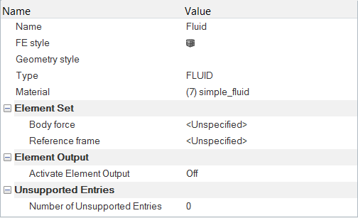
Figure 9. -
Click Inflow. In the Entity Editor,
- Change the Type to INFLOW.
- Turn On the Show advanced features field.
- Set the Normal velocity to 0.1 m/sec.
- Set the Temperature to 300 K.
- Set the Temperature multiplier function to inflow_temperature_control.
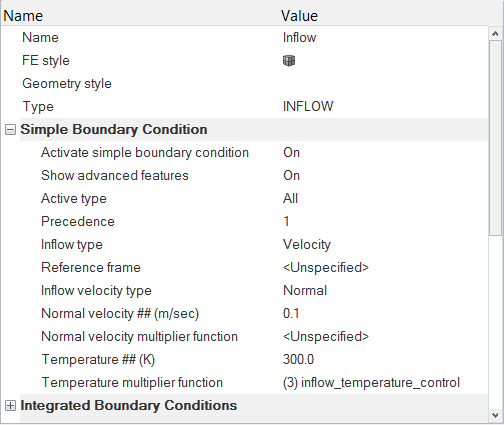
Figure 10. -
Click Outflow. In the Entity Editor, change the Type to
OUTFLOW.
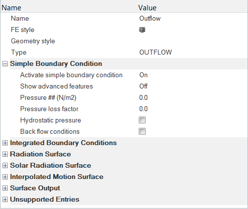
Figure 11. -
Click Outer_Walls. In the Entity Editor, change the Type to
SLIP.
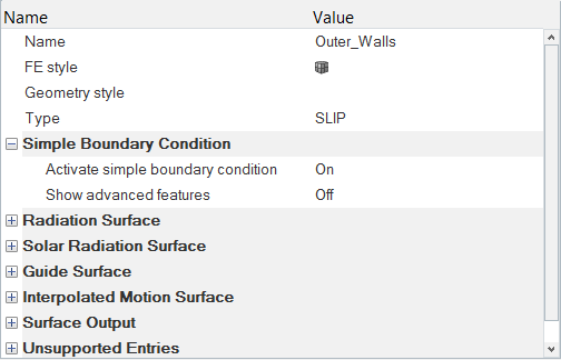
Figure 12. -
Click Sphere_Wall. In the Entity Editor,
- Change the Type to WALL.
- Change the Temperature BC type to Value.
- Set the Temperature to 500 K.
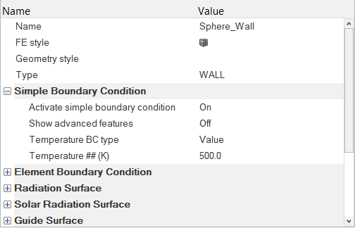
Figure 13.
Compute the Solution and Review the Results
Run AcuSolve
In this step, you will launch AcuSolve directly from HyperMesh and compute the solution.
-
In the Model Browser, ensure that the visibility of the
mesh for all collectors to be exported for AcuSolve
are activated. In this case, display for all the collectors – Fluid, Inflow,
Outflow, Sphere_Wall, and Outer_Walls – should be activated.
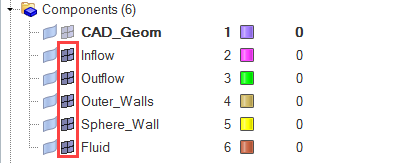
Figure 14. -
Click
 on the ACU toolbar.
The Solver job Launcher dialog opens.
on the ACU toolbar.
The Solver job Launcher dialog opens.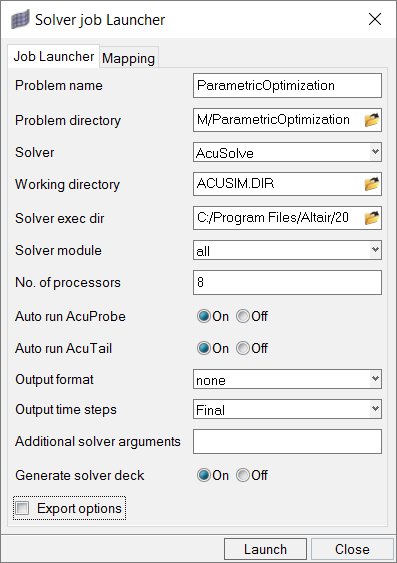
Figure 15.For this case, the default settings will be used. You may choose to change the number of processors to allow AcuSolve to run using more processors (4 or 8), if available. HyperMesh will generate the required solver input files and launch AcuSolve. AcuSolve will calculate the steady state solution for this problem.
-
Click Launch to start the
solution process.
As the solution progresses, an AcuTail and an AcuProbe dialog will open. Solution progress is reported in the AcuTail dialog. An AcuSolve Control dialog will also open from which you can control the solution process. In this dialog you have options to stop the solution or generate the output files at the end of the current time step.You'll notice AcuSolve prints the case number before beginning the solution for the case. The Case-Step number is reset to 1 when AcuSolve moves to a new case while Time-Step proceeds sequentially.
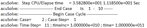
Figure 16.A summary of the run printed in the AcuTail dialog indicates that AcuSolve has finished running the solution.
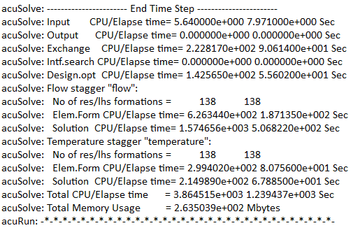 Figure 17.
Monitor the Solution with AcuProbe
AcuProbe can be used to monitor various variables over solution time. An AcuProbe window will be launched by the Solver Job Launcher if the Auto run AcuProbe flag is set to On.
-
Right-click on temperature and select
Plot.
Note: You might need to click
 on the toolbar in order to
properly display the plot.
on the toolbar in order to
properly display the plot.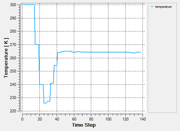
Figure 18.This plot shows the surface temperature of the inflow surface as the solution progresses.
In the setup, the inflow temperature is a design variable. At the inflow surface, the temperature varies from case to case in accordance with the values provided to the solver by the optimization program. The first three values of inflow temperature correspond to the values provided in the supervised learning parameter, after which the values are provided by the optimizer. The converged value of the inflow temperature is approximately 264.15 K. This is the value at which the outflow temperature is closest to its target value.
-
Right-click on temperature and select
Plot.
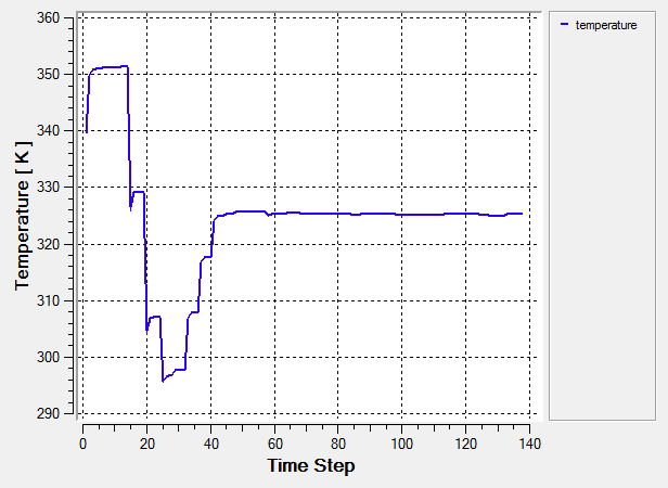
Figure 19.This plot shows the surface temperature of the outflow surface as the solution progresses.
At the outflow surface, the temperature varies in the beginning of the simulation and ultimately converges to a value close to the target temperature value, i.e. 325 K.
AcuGetDv and AcuGetRsp
AcuSolve provides two post-processing utilities specific to optimization problems, AcuGetDv and AcuGetRsp. AcuGetDv provides the values of the design variables for all the cases included in the solution. AcuGetRsp provides the values of the response variables for all the cases included in the solution.
-
Enter the following command at the prompt:
acuGetDv
AcuSolve will print the values of design variables for each case.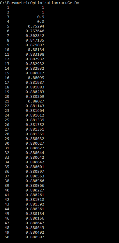
Figure 20. -
To print the values of response variables, use the command:
acuGetRsp
Note: The order of columns in which the design variables and the response variables are printed by these commands is the order in which they appear in the INP file.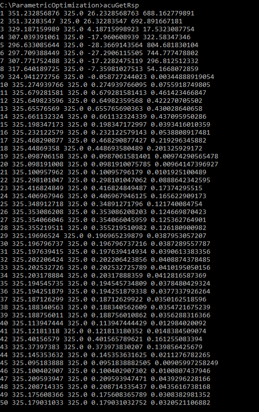
Figure 21.
Summary
In this AcuSolve tutorial, you successfully set up and solved a parametric optimization problem with AcuSolve. You started the tutorial by creating a database in HyperMesh, importing and meshing the geometry, and setting up the simulation parameters. You defined the design variables, the response variables, and set up the objectives of the problem using the response variables. Once the case was setup, the solution was generated with AcuSolve. AcuProbe was used to visualize the variation of design variables and response variables as the solution progressed through the different cases provided to AcuSolve by the optimization program. You also used the utilities provided in AcuSolve to get the design variables and response variables information for all the cases.