ACU-T: 6100 Particle Separation in a Windshifter using Altair EDEM
This tutorial introduces you to the workflow for setting up and running a basic sequential coupling (one-way steady) simulation using AcuSolve and EDEM. Prior to starting this tutorial, you should have already run through the introductory HyperWorks tutorial, ACU-T: 1000 HyperWorks UI Introduction, and have a basic understanding of HyperWorks CFD, AcuSolve, and EDEM. To run this simulation, you will need access to a licensed version of HyperWorks CFD, AcuSolve, and EDEM.
Prior to running through this tutorial, copy HyperWorksCFD_tutorial_inputs.zip from <Altair_installation_directory>\hwcfdsolvers\acusolve\win64\model_files\tutorials\AcuSolve to a local directory. Extract ACU-T6100_windshifter.hm from HyperWorksCFD_tutorial_inputs.zip.
Problem Description
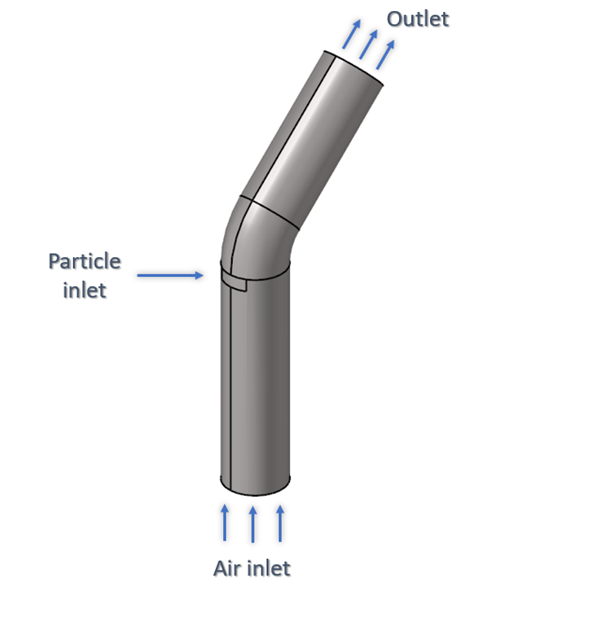
Figure 1.
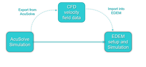
Figure 2.
The tutorial consists of two parts:
- AcuSolve simulation
- EDEM simulation
The setup for the AcuSolve simulation is done using HyperWorks CFD. Once the AcuSolve simulation is complete, the velocity nodal data is exported into CGNS format using the AcuTrans utility available in AcuSolve. This field data will be imported into EDEM and will be used to calculate the drag forces on the particles due to the fluid.
Two different bulk materials used in the EDEM simulation and their properties are listed below:
| Name | Density (kg/m3) | Size of particle (m) | Average weight of individual particle (kg) | Rate of generation (particles per sec) |
|---|---|---|---|---|
| Heavy particle | 900 | 0.01 | 0.004 | 100 |
| Light particle | 100 | 0.01 | 0.0004 | 100 |
The fluid drag forces on the particles are calculated using the Schiller-Naumann drag model. The drag force on the particle is calculated using the relative velocity of the particle with respect to the local fluid velocity. This particle body force will used to update the location of the particles and then the new drag forces are calculated. This loop is repeated until the end of the simulation.
Part 1 - AcuSolve Simulation
Start HyperWorks CFD and Open the HyperMesh Database
-
From the Home tools, Files tool group, click the Open Model tool.

Figure 3.The Open File dialog opens.
Validate the Geometry
The Validate tool scans through the entire model, performs checks on the surfaces and solids, and flags any defects in the geometry, such as free edges, closed shells, intersections, duplicates, and slivers.
Figure 4.
Set Up Flow
Set the General Simulation Parameters
-
From the Flow ribbon, click the Physics tool.

Figure 5.The Setup dialog opens. -
Under the Physics models setting:
- Verify that the Incompressible option is selected under Single phase flow.
- Activate the Export geometry to EDEM check-box.
- Set Time marching to Steady.
- Select Spalart-Allmaras as the Turbulence model.
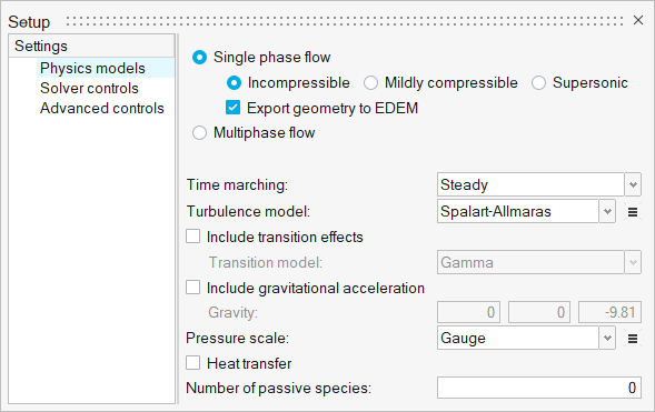
Figure 6.
Assign Material Properties
-
From the Flow ribbon, click the Material tool.

Figure 7. -
On the guide bar, click
 to exit
the tool.
to exit
the tool.
Define Flow Boundary Conditions
-
From the Flow ribbon, Profiled
tool group, click the Profiled Inlet tool.

Figure 8. -
Click on the inlet face highlighted in the figure below and enter a value of
20 m/s for the Average velocity in the microdialog.
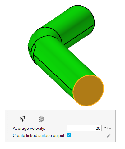
Figure 9. -
On the guide bar, click
 to execute
the command and exit the tool.
to execute
the command and exit the tool.
-
Click the Outlet tool.

Figure 10. -
Select the face highlighted in the figure below then click on the
guide bar.
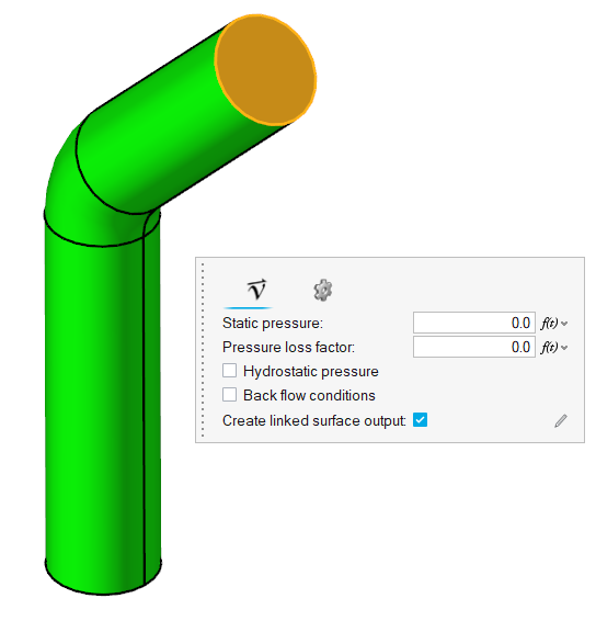
Figure 11. -
Click the No Slip tool.

Figure 12. -
Select the face highlighted in the figure below.
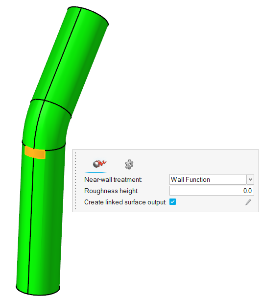
Figure 13. -
Click on the guide bar.
Generate the Mesh
-
From the Mesh ribbon, click the
Volume tool.

Figure 14.The Meshing Operations dialog opens.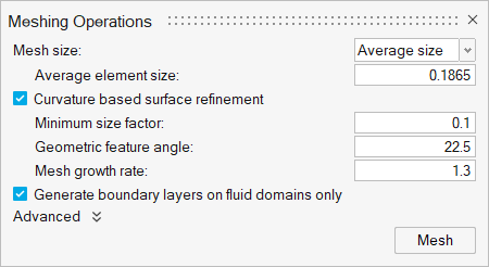
Figure 15.
Run AcuSolve
-
From the Solution ribbon, click the Run tool.

Figure 16.The Launch AcuSolve dialog opens. -
Click Run to launch AcuSolve.
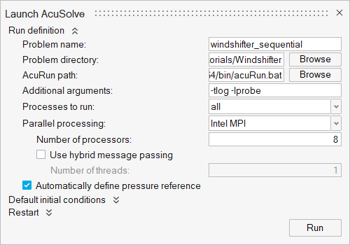
Figure 17.Once the AcuSolve simulation is launched, HyperWorks CFD also exports the EDEM files which contain the geometry. The surfaces are organized based on the CFD setup.
Export Velocity Field Data
As the solution progresses, the AcuTail and AcuProbe windows are launched automatically.
In the AcuTail window, the residual ratio and solution ratio information is printed as the simulation progresses.
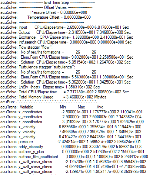
Figure 18.
-
From the Solution ribbon, click the
Convert tool.

Figure 19.The AcuSolve Data Translator dialog opens. -
Click Convert to export the velocity nodal data in CGNS
format.
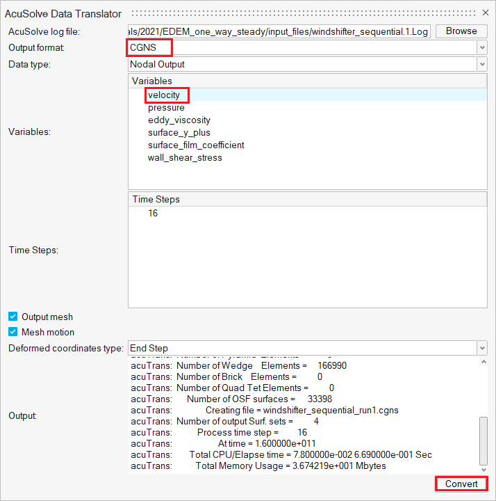
Figure 20.Once the process is successful, the same information is printed in the Output field and a CGNS file is created in the AcuSolve problem directory.
Post-Process the Results with HW-CFD Post
-
Select the Left face on the view cube to align the model
to the x-z plane.
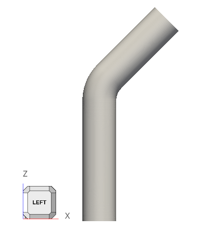
Figure 21. -
In the Post Browser, turn off the display of the boundary
surfaces by clicking on the icon next to Flow Boundaries.
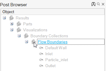
Figure 22. -
Click the Slice Planes tool.

Figure 23. -
In the slice plane microdialog, click
 to
create the slice plane.
to
create the slice plane.
-
Click
 and set the Colormap name to Rainbow
Uniform.
and set the Colormap name to Rainbow
Uniform.
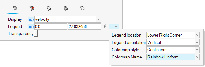
Figure 24. -
Click on the guide bar.
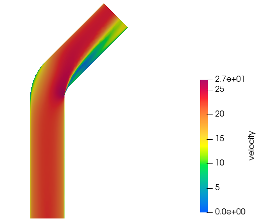
Figure 25.
Part 2 - EDEM Simulation
Start Altair EDEM from the Windows start menu by clicking . The user interface in EDEM is divided into three tabs: Creator, Simulator and Analyst. The Creator is used to setup and initialize your model. It is where you import particles and geometries and define the other model parameters. The Simulator is where you configure and control the EDEM simulation engine, and where you can observe the progress of your simulation. The Analyst is the post-processor used to analyze and visualize the results of your simulation.
The steps required to setup and run a basic CFD-DEM one-way coupling are explained below. Please refer to the EDEM help documentation for more details.
Open the EDEM Input Deck
As mentioned earlier, when the AcuSolve simulation was launched, HyperWorks CFD created a set of EDEM files in the problem directory. You will open that EDEM input deck and setup the DEM simulation
-
Click the Environment tab under the Creator Tree,
uncheck Auto Update from Geometry, then check the box
again to fit the geometry within the boundary.
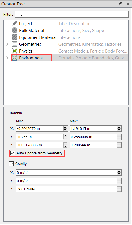
Figure 26.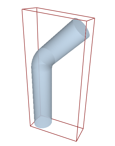
Figure 27.
Define the Bulk Materials and Equipment Material
In this step, you will define the material models for the heavy and light bulk material and the equipment material.
-
In the Creator Tree, set the Solids Density property to
900 kg/m3.
You will use the default values for other properties for this tutorial.
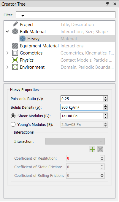
Figure 28. -
Click
 below Interaction to define the
interaction properties for collisions among the heavy particles. In the dialog,
click OK.
below Interaction to define the
interaction properties for collisions among the heavy particles. In the dialog,
click OK.
-
In the Heavy particle Spheres panel, set the Physical Radius of both the
spheres to 0.03 m and press Enter.
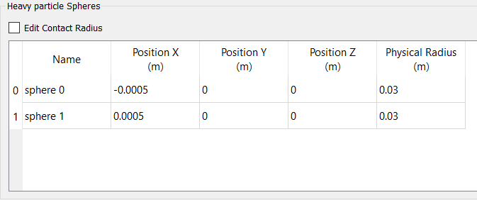
Figure 29. -
In the Creator Tree, click Calculate Properties.
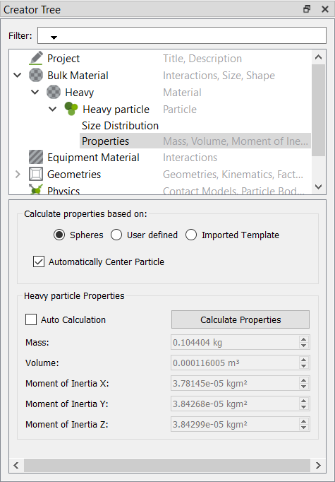
Figure 30. -
In the Creator Tree, set the Solids Density property to
100 kg/m3.
You will use the default values for other properties for this tutorial.
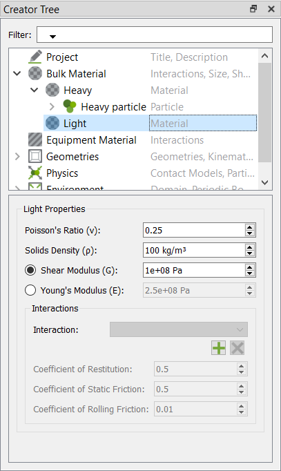
Figure 31. -
Click below Interaction to define the
interaction properties for collisions among the heavy particles. In the dialog,
select Heavy then click OK.
-
Click again to define the interaction
properties for collisions among the light particles. In the dialog, select
Light then click OK.
-
In the Light particle Spheres panel, set the Physical Radius of both the
spheres to 0.03 m and press Enter.
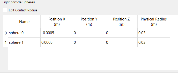
Figure 32. -
In the Creator Tree, click Calculate Properties.
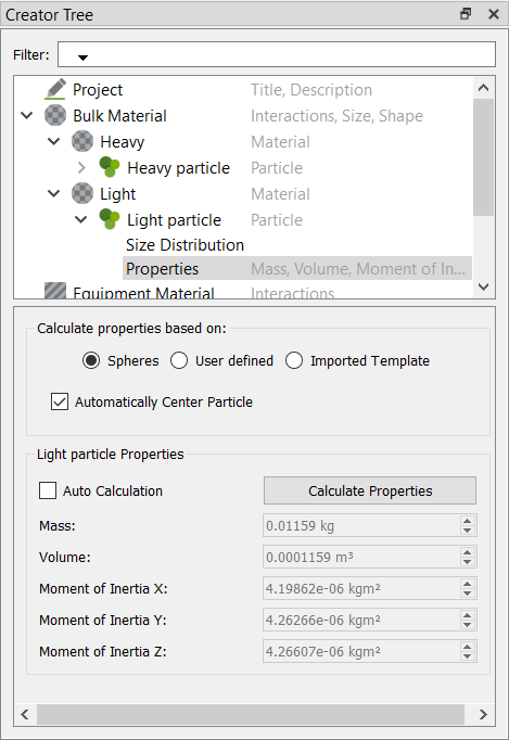
Figure 33. -
Click below Interaction to define the
interaction properties for collisions among the heavy particles. In the dialog,
select Heavy then click OK.
-
Click again to define the interaction
properties for collisions among the light particles. In the dialog, select
Light then click OK.
Create the Particle Factory
-
Click on the Default Wall geometry section, set the Type
to Physical, and the Material to
Steel (if not set already).
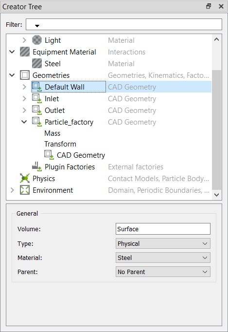
Figure 34. -
Under Particle_factory, click Transform. Set the
X-Position to 0.035 m
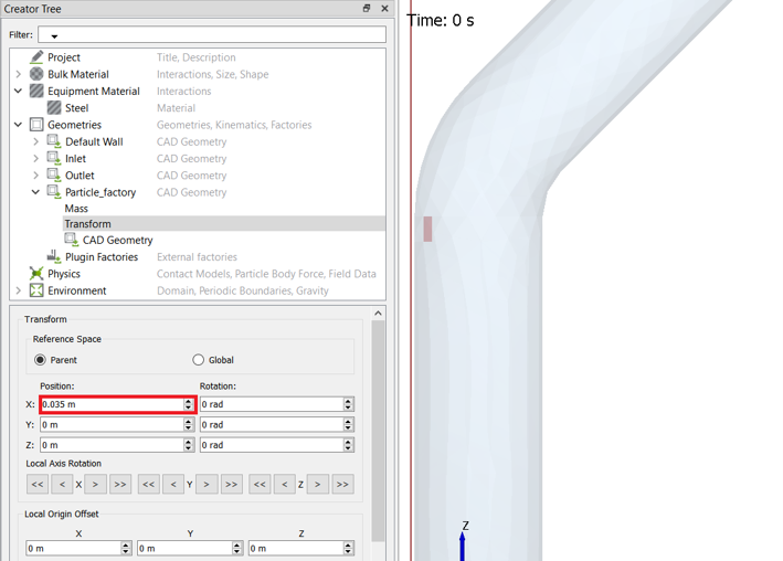
Figure 35.Note: Set the Opacity value to 0.2 to see the transformed surface location inside the pipe geometry.This is done to make sure that the particles are generated inside the fluid domain.
Define the Particle Factory
Now that the bulk material, geometry sections, and equipment materials are defined, you need to create a particle factory to generate the particles. You will create one factory for each bulk material.
-
Set the particle generation parameters as shown in the figure below.
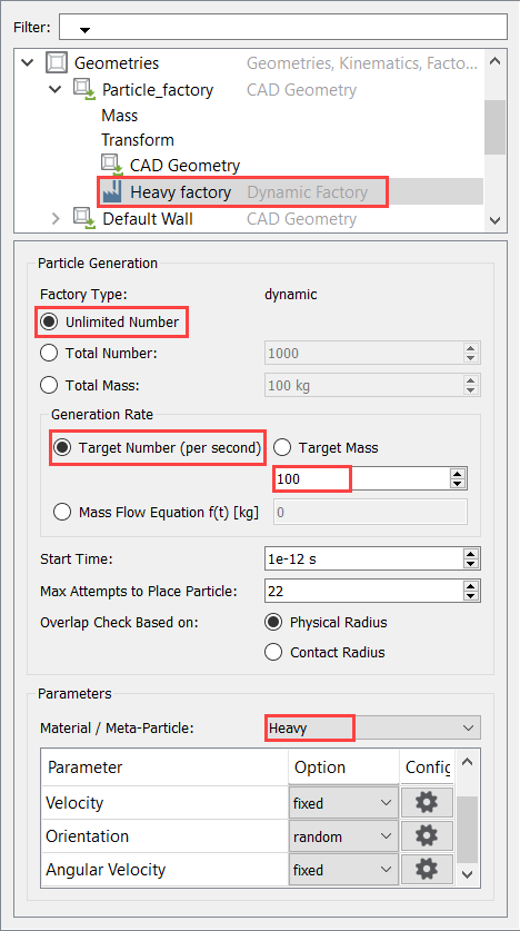
Figure 36. -
Click
 besides Velocity, set the
X-velocity to 1 m/s, then click
OK.
besides Velocity, set the
X-velocity to 1 m/s, then click
OK.
Define the Physics and Import CFD Field Data
In this step, you will define the physics models for particle collisions and the particle body force.
-
Click the Interaction drop-down menu and select
Particle Body Force.
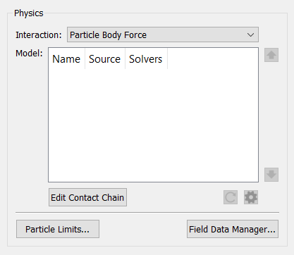
Figure 37. -
In the Physics tab, click on Schiller and Naumann Drag
then click .
-
In the Schiller and Naumann Drag Parameter Values dialog,
enter the values as shown in the figure below then click
OK.
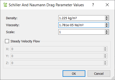
Figure 38. -
In the Field Data Manager
dialog, click then browse to the AcuSolve problem directory where you saved the CGNS file
exported using the CFD field data. Open
windshifter_sequential_run1.cgns.
-
Once the data import is complete, double-click on
Velocity and rename it to
velocity. (The letter ‘v’ should be in lower case).
Then, close the dialog.
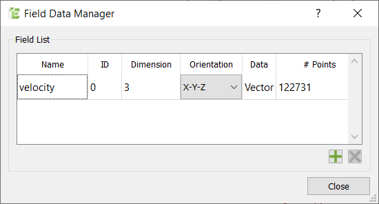
Figure 39.
Define the Environment
In this step, you will define the extents of the domain for the EDEM simulation and the direction of gravitational acceleration.
Define the Simulation Settings and Run the Simulation
-
Click
 in the top-left corner to go to
the EDEM Simulator tab.
in the top-left corner to go to
the EDEM Simulator tab.
-
Set the Selected Engine to CPU Solver and set the Number
of CPU Cores based on availability.
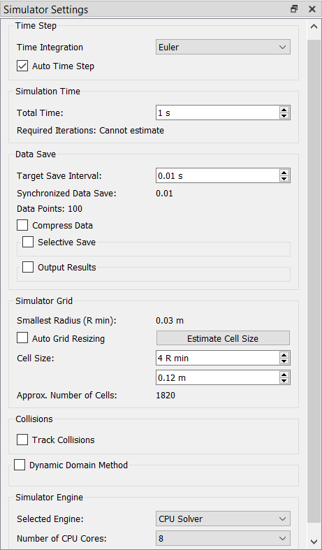
Figure 40. -
Once the simulation settings have been defined, click
 to start the EDEM simulation.
Analyze the Results
-
Once the EDEM simulation is complete, click
 in the top-left corner to go to
the EDEM Analyst tab.
in the top-left corner to go to
the EDEM Analyst tab.
-
Verify that the Display Mode is set to Filled and set
the Opacity to 0.2.
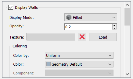
Figure 41. -
Change the display color to Magenta.
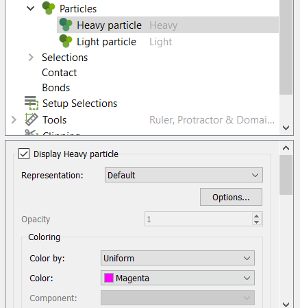
Figure 42. -
Click on Light particle and set the display color to
Green.
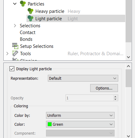
Figure 43. -
On the menu bar, set the time to
0 by clicking:

Figure 44. -
Set the View plane to + Y.
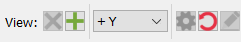
Figure 45. -
In the Viewer window, set the Playback Speed to 0.1x
then click on the play icon to play the particle flow animation.
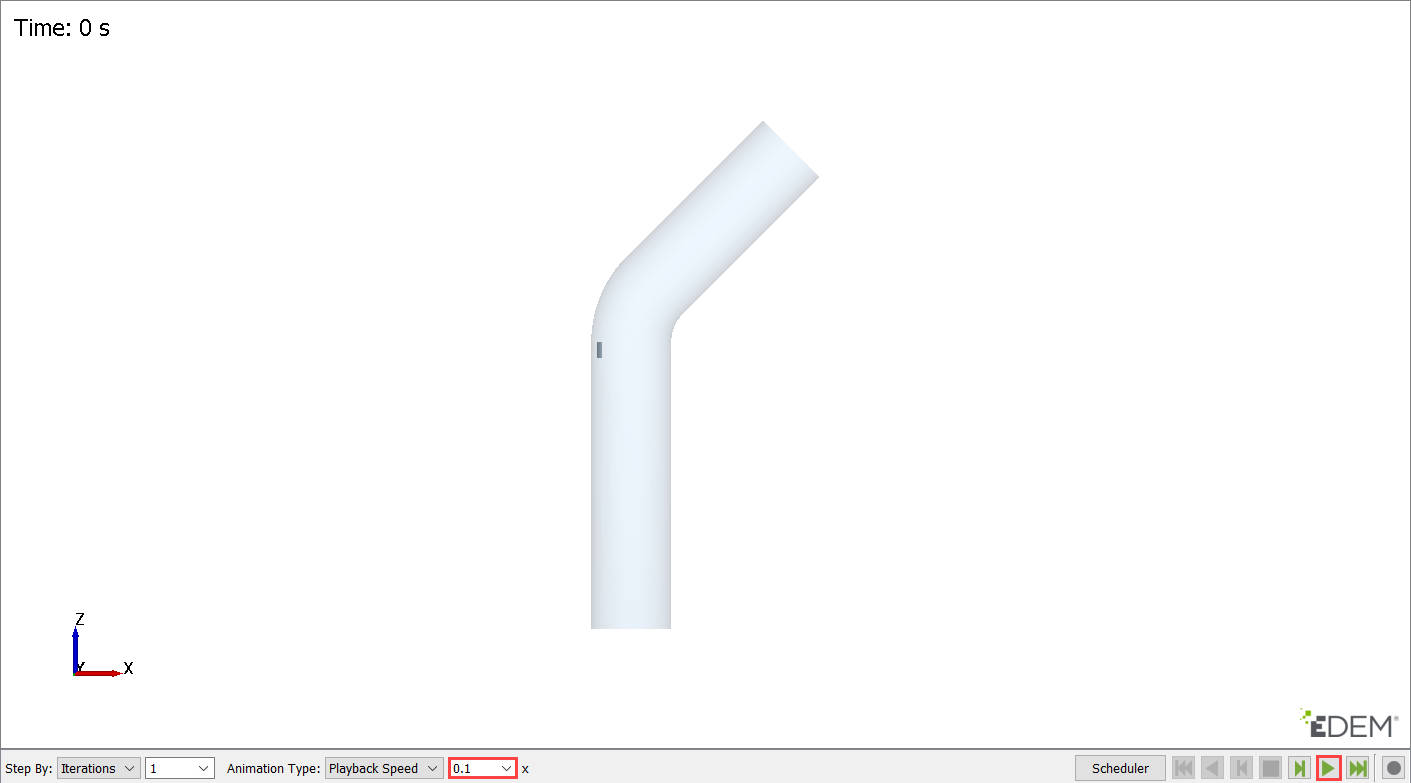
Figure 46.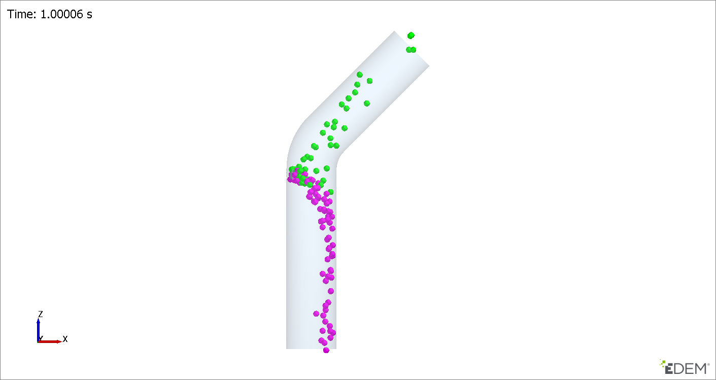
Figure 47.Observe that the lighter particles (green) get carried by the fluid and escape the domain through the outlet at the top and the heavier particles (magenta) stay inside the domain for a longer time while some of them fall through the bottom of the pipe.
Summary
In tutorial you learned how to setup a basic AcuSolve-EDEM sequential (one-way steady) coupling problem. In the first part, you set up and solved a steady state flow simulation using AcuSolve and then exported the CFD field data using AcuTrans. Next, you set up the EDEM model and imported the CFD field data using the Field Data Manager. Once the EDEM simulation was completed, you learned how to view results and create animations in EDEM Analyst.