ACU-T: 5402 Piezoelectric Flow
Energy Harvester with Rigid Body Rotation
This tutorial provides the instructions for setting up, solving and viewing results for a
simulation of a piezoelectric fluid harvester. In this simulation, a piezoelectric flow
harvester is placed in a fluid flow channel. The harvester is attached to a cylinder mount
which also acts as a bluff body causing vortices in the fluid flow. In addition, the
cylinder and the harvester are imparted with a sinusoidal rotation motion. The interaction
between the pressure fields generated by the vortices and the flow harvester structure is
simulated in this tutorial. Arbitrary Lagrangian Eulerian (ALE) approach is used to compute
the mesh deformation in the fluid domain as it interacts with the deforming structure.
The basic steps in any CFD simulation are shown in ACU-T: 2000 Turbulent Flow in a Mixing Elbow. The following additional
capabilities of AcuSolve are introduced in this
tutorial:
Defining rigid body rotation motion
Implementation of P-FSI in conjunction with rigid body rotation
In this tutorial you will do the following:
Analyze the problem
Start AcuConsole and read the simulation database of the
Piezoelectric Flow Harvester
Modify general problem parameters
Create multiplier function for rigid body mesh motion
Create mesh motion for rigid body rotation
Apply mesh motion to the surface attributes
Assign rigid body motion to the surface and node attributes
Change the inlet velocity
Add a time history output point
Run AcuSolve
Monitor the solution with AcuProbe
Post-processing the nodal output with AcuFieldView
Prior to running through this tutorial, copy
AcuConsole_tutorial_inputs.zip from
<Altair_installation_directory>\hwcfdsolvers\acusolve\win64\model_files\tutorials\AcuSolve
to a local directory. Extractpiezo_harvester_P-FSI.acsfrom AcuConsole_tutorial_inputs.zip. The file piezo_harvester_P-FSI.acs stores the complete setup as described in
Piezoelectric Flow Harvester, which includes purely flexible body simulation.
In this tutorial, you will start from that database and add a rigid body rotation and then
simulate the flow phenomenon.
Analyze the Problem
An important step in any CFD simulation is to examine the engineering problem at hand and
determine the important parameters that need to be provided to AcuSolve.
The CFD model contains a cantilever beam and a rigid cylindrical body. The beam along with the
cylinder is placed in a water flow stream. This cylindrical body acts a bluff body placed in the
flow and stimulates vortex shedding in the flow downstream as it passes over the cylinder. The
alternating shedding of vortices creates a zone of alternating asymmetric pressure distribution
on either side of the beam. Such an alternating pressure distribution exerts an oscillating force
on the beam, creating a sustainable oscillating vibration in the beam.
In this tutorial, in the addition to the flexible motion of the beam adopted in Piezoelectric
Flow Harvester Tutorial-1, you will incorporate the rigid body rotation of the cylinder and the
beam. The cylinder and the beam are enforced with a sinusoidal oscillatory rotation about the
center of the cylinder with a maximum angle of rotation as 100 (i.e. 0.174 rad) with a frequency
of 22 rad/sec (3.5 Hz). The axis of rotation is along axis of cylinder. The variation of the
rotation angle (θ) is given as:
Where, t is the time (sec).
Since this tutorial has a rotation motion in addition to flexible motion of beam, you can
achieve higher displacements (and hence strains) at lower velocity. Therefore, you will reduce
the inlet velocity to 4 m/sec instead of 10 m/sec in Piezoelectric Flow Harvester Tutorial-1.
The schematics of the problem which will be addressed in this tutorial is shown in Figure 1. The modeled domain
consists of a fluid volume. The fluid solver does not require the solid body to be modeled.
However, the results of the structural solver will be used to define the solid body and the
surfaces where the fluid interacts with the solid will be allowed to deform according to the
Eigen modes of the beam. Figure
2 shows the arrangement of the beam with its various layers. Figure 1. Schematic of the Problem
Figure 2. The Beam with its Various Layers
Define the Simulation Parameters
Start AcuConsole and Open the Simulation Database
In the next steps you will start AcuConsole and open a
database that is set up for a P-FSI simulation of a non-rotating piezoelectric
harvester. You will then make appropriate changes to the database to take into
account the rigid body rotation of the harvester in addition to the flexible body
motion.
Start OptiStruct from the Windows Start menu by
clicking Start > Altair <version> > OptiStruct.
Browse to the location that you would like to use as your working
directory.
This directory is where all files related to the simulation will
be stored. The AcuConsole database file
(.acs) is stored in
this directory. Once the mesh and solution are created, additional files and
directories will be created within this directory.
Create a new directory in this location. Name it
P-FSI_with_rigid_body_motion.
Click File > Open and open piezo_harvester_P-FSI.acs.
Click File > Save As and enter P-FSI_with_rigid_body_rotation
as the file name for the database.
Set General Simulation Attributes
In the next steps you will modify global settings needed for
the rigid body rotation of the piezoelectric harvester.
Click BAS in the Data Tree Manager to switch to basic view in the Data Tree.
Figure 3.
Double-click the GlobalData Tree item to expand it.
Tip: You can also expand a tree item
by clicking
next to the item name. Figure 4.
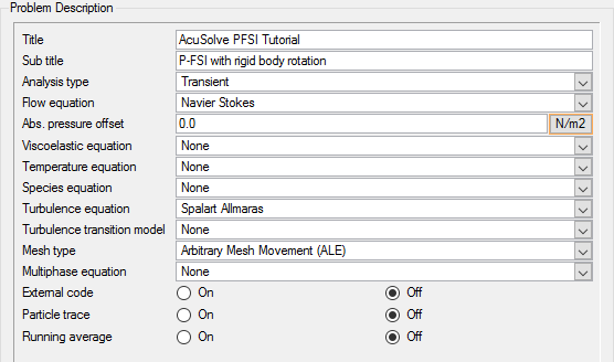
Double-click Problem
Description to open the Problem
Description detail panel.
Tip: You can also open a panel by right-clicking a tree item and
clicking Open on the context menu.
Enter P-FSI with rigid body rotation as the Sub
title.
Figure 5.
Create a Multiplier Function for Mesh Motion
The variation of the rotation angle () is modeled using a multiplier function using the
following steps.
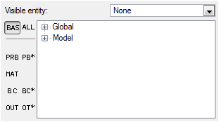
Click PB* in the Data Tree Manager to display all the available settings related to general problem setup in
the Data Tree.
Right-click Multiplier Function and click New
to create a new multiplier function.
A new entry, Multiplier Function 1, will be created in the Data Tree under the Multiplier Function branch.
Rename the new multiplier function.
Right-click Multiplier Function 1.
Click Rename.
Type Rotation_multiplier and press Enter.
Double-click Rotation_multiplier to open the detail
panel.
Change Type to Sine Series.
Click Open Array next to Sine coefficients.
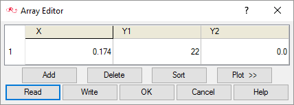
Fill in the values as follows:
In the Array Editor, the first column refers to the
amplitude of the sine function, second column refers to the frequency of the
sine function and the third column refers to phase of the sine wave. Figure 6.
Click OK to close the dialog.
Create Mesh Motion for Rigid Body Rotation
In the next steps you will define the rigid body rotation of the cylinder and the
beam.
Click ALE in the Data Tree Manager to see all the settings related to mesh motion.
Right-click Mesh Motion and click New
to create a new mesh motion.
Rename the new reference frame as
Rigid_body_rotation.
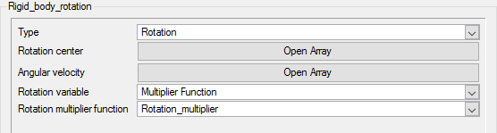
Double-click Rigid_body_rotation to open the detail
panel.
Change the Type to Rotation.
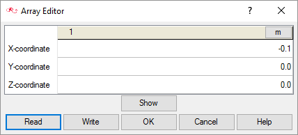
Click the Open Array button next to Rotation center to
open the Array Editor.
Enter -0.1 as the X-coordinate.
Figure 7.
Click OK to close the dialog.
Note: (x, y, z) = (-0.1, 0, 0) is the center of the cylinder.
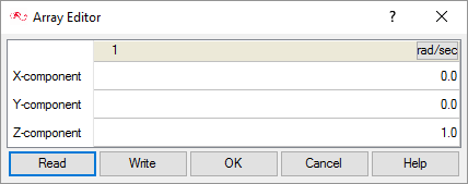
Click the Open Array button next to Angular velocity to
open the Array Editor.
Enter 1.0 as the Z-coordinate.
Figure 8.
Click OK to close the dialog.
Set the Rotation variable to Multiplier Function.
Set the Rotation multiplier function to
Rotation_multiplier.
Figure 9.
Using the mesh motion Type = Rotation defines the variation of the rotation
angle which is used by AcuSolve in evaluating
the coordinates of the beam and cylinder. The rotation angle is evaluated by
multiplying the value of Rotation Variable with the components of Angular
Velocity. Therefore, for this tutorial, the rotation angle comes out to
be:(1)
about z-axis
For a point with initial coordinates, located on the cylinder or beam, the
coordinates at a given time, t, is given by:(2)(3)(4)
Assign Rigid Body Motion to the Beam Surface
Click BAS in the Data Tree Manager to switch to basic view in the Data Tree.
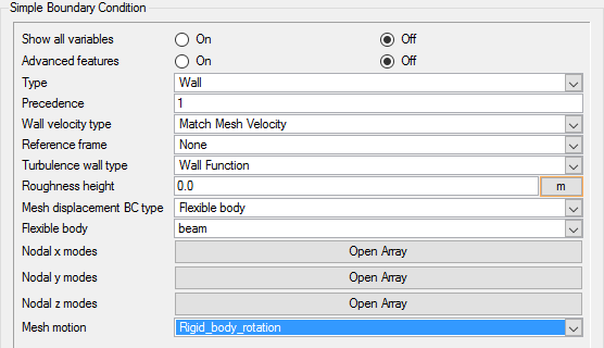
Expand Model > Surfaces > Beam.
Double-click Simple Boundary Condition to open the
detail panel.
Set the Mesh motion to Rigid_body_rotation.
Figure 10.
Assign Rigid Body Motion to the Cylinder Surface
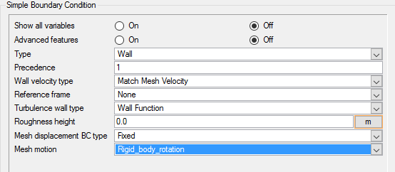
Expand Model > Surfaces > Cylinder.
Double-click Simple Boundary Condition to open the
detail panel.
Set the Mesh motion to Rigid_body_rotation.
Figure 11.
Click Save to save the database.
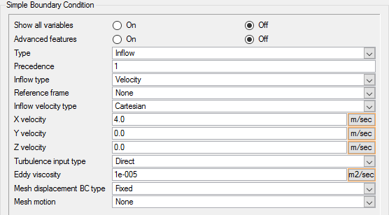
Reduce the Inlet Velocity
As mentioned in Analyze the Problem,
you will set the inlet velocity to 4 m/sec.
Expand Model > Surfaces > Inlet.
Double-click Simple Boundary Condition to open the
detail panel.
Set the X velocity to 4.0 m/sec.
Figure 12.
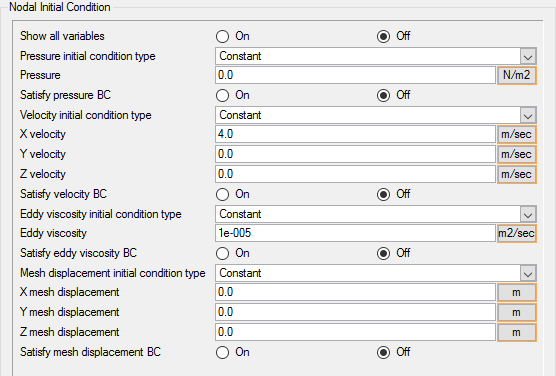
Set Initial Conditions
In the next steps you will set the initial conditions.
Under Global in the Data Tree, double-click
Nodal Initial Condition to open the dialog in the
detail panel.
Set the X velocity to 4 m/sec.
Verify that the Eddy viscosity is set to 1e-005
m2/sec.
Figure 13.
Save the database.
Add Time History Output Point
Time History Output commands enables you to extract the nodal solution at any point
within the domain. In this simulation, it would be interesting to observe the
displacement at the tip and root of the cantilever beam. The
.acs database you started with has a monitor point at the
tip of the cantilever beam.
The following steps will create a similar monitor point at the root of the cantilever
beam.
Double-click the GlobalData Tree item to expand it.
Double-click Output.
Right-click on Time History Output, and select
New.
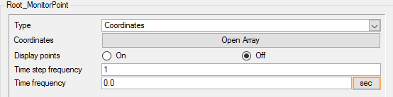
Rename the new time history output to
Root_MonitorPoint.
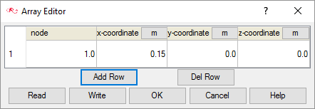
Double-click Root_MonitorPoint to open the detail
panel.
Change the Type to Coordinates.
Click Open Array next to Coordinates, and update the
fields in the Array Editor dialog, as follows:
Figure 14.
Set Time step frequency to 1.
Click Save to save the database.
Figure 15.
Compute the Solution and Review the Results
Run AcuSolve
In the next steps you will launch AcuSolve to compute the solution for this case.
Click on the toolbar to open the
Launch AcuSolve dialog.
Click Ok to start the
solution process.
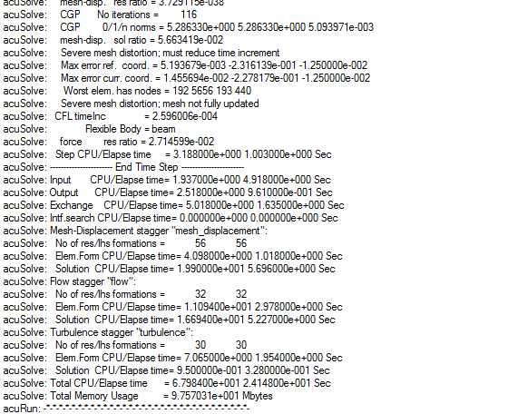
While computing the solution, an
AcuTail window opens. Solution progress is
reported in this window. A summary of the solution process indicates
that the run has been completed.
The information provided in the summary is based on
the number of processors used by AcuSolve.
If you use a different number of processors than indicated in this
tutorial, the summary for your run may be slightly different than the
summary shown.
Figure 16.
Close the AcuTail window and save the database to create a
backup of your settings.
Post-Process with AcuProbe
AcuProbe can be used to monitor various variables over
solution time.
Open AcuProbe by clicking on the toolbar.
In the Data Tree on the left, expand Time History > Root_MonitorPoint > node 1.
Right-click on mesh_y_displacement and select
Plot.
Note: You might need to click on the toolbar in order to
properly display the plot.
Repeat the above steps to plot the mesh_y_displacement for the
Tip_MonitorPoint.
Figure 17.
The plot above shows the displacement of the tip and the root of the beam,
due to the fluid forces as the beam interacts with the flow. The above plot
also shows the displacement at the root and at the tip are not in phase,
hence maximizing the bending stress (hence, strains) for a lower inlet
velocity.
You can also save the plots as an image.
From the AcuProbe dialog, click File > Save.
Enter a name for the image and click
Save.
The time series data of the variables can also be exported as a text file
for further post-processing.
Right-click on the variable that you want to export and click
Export.
Enter a File name and choose .txt for
the Save as type.
Click Save.
Post-Process with AcuFieldView
The tutorial has been written with the assumption that you have become familiar
with AcuFieldView and basic operations. In general, it will
be helpful to understand the following basics:
How to find the data readers in the File menu and open up the desired reader
panel for data input.
How to find the visualization panels either from the Side toolbar or the
Visualization panel on the Main menu to create and modify surfaces in AcuFieldView.
How to move the data around the modeling window using
mouse actions to translate, rotate and zoom in to the data.
Start AcuFieldView
Click on the
AcuConsole toolbar to open the
Launch AcuFieldView dialog.
You will see that the pressure contours have already been displayed on
all of the boundary surfaces with mesh. When results of a transient simulation
are loaded in AcuConsole, the displayed results
correspond to the last time step of the simulation. Figure 18.
Set Up AcuFieldView
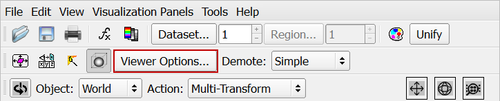
Close the Boundary Surface dialog.
Click Viewer Options.
Figure 19.
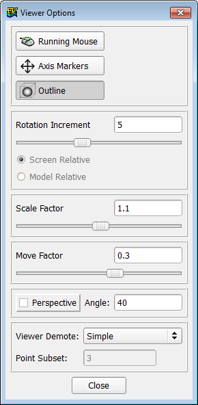
In the Viewer Options dialog:
Turn off perspective view by deselecting the
Perspective check box.
Disable the axis markers by clicking Axis
Markers.
Figure 20.
Click Close to close the dialog.
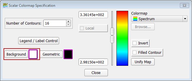
Click the Scalar Colormap Specification icon on the toolbar.
In the Scalar Colormap Specification dialog, click
Background.
Figure 21.
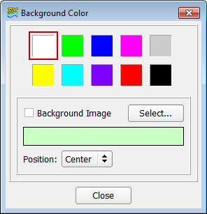
In the Background Color dialog, select the color
white.
Figure 22.
Close the dialogs.
Click the icon to turn off the outline
display.
Your model should now look like this: Figure 23.
Visualize and Save an Animation of the Beam Displacement
Click to open the Boundary
Surface dialog.
Turn off the visibility for the active boundary surfaces.
Click to open
the Coordinate Surface dialog.
Create a new coordinate surface at the mid -Z coordinate plane.
The coordinate surface created is the mid plane between the z_neg and
z-pos surfaces.
Set the Coloring to Scalar.
Set the Display Type to Smooth.
Select x-velocity as the Scalar Function to be
displayed.
Select Z as the Coord Plane.
In the Colormap tab, change Scalar Coloring to
Local.
From the Defined Views, select +Z as the viewing
direction.
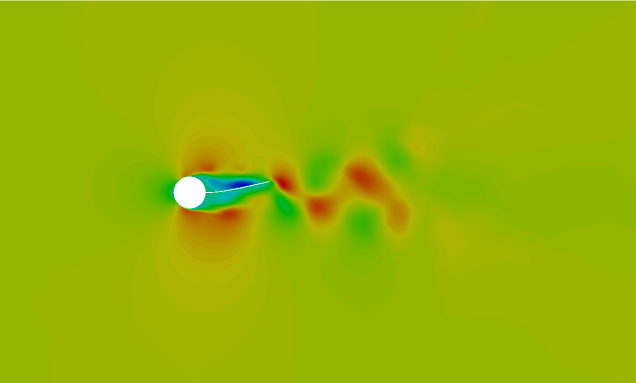
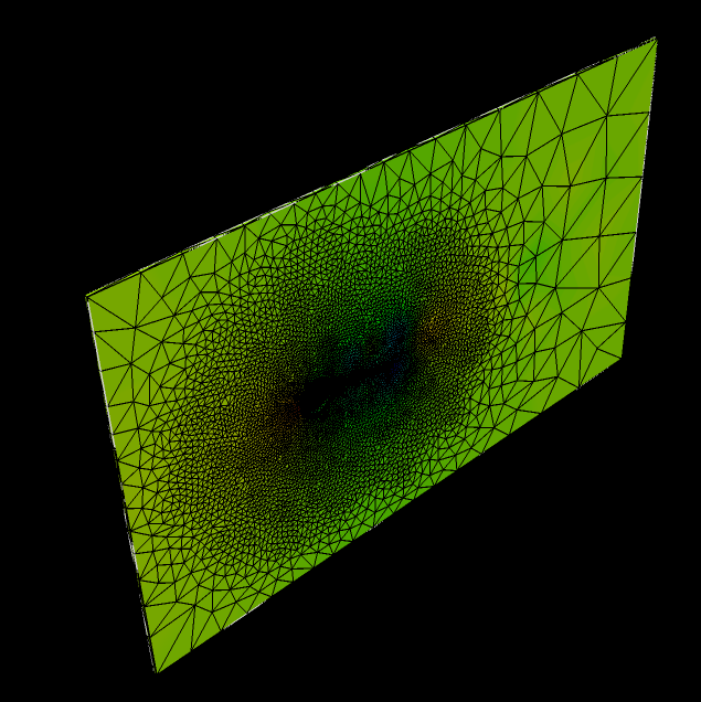
Your model should look like the image below. The visible shape of the
beam is its deformed shape at the end of last time step in the simulation. Figure 24.
Close the dialog.
Click Tools > Flipbook Build Mode.
Click OK to close the Flipbook Size
Warning dialog.
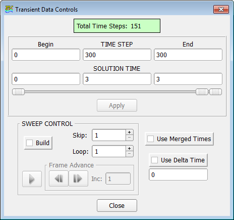
Click Tools > Transient Data.
The Transient Data Controls dialog opens. Figure 25.
If the Sweep Control in this dialog shows Sweep instead of Build, the
Flipbook Build mode is not active. In Sweep mode, you will be able to create and
visualize the animation, but you will not be able to save it. To be able to save
the animation, enable the Flipbook Build Mode.
Drag the time step slider to its left most position. Alternatively, type
0 for the Time Step or Solution Time.
Click Apply.
The displayed state now corresponds to the initial state of the
domain. Figure 26.
Click Build.
AcuFieldView will build the frame by
frame animation of the solution progressing through all of the available
time steps. You will be able to see the progress in a Building
Flipbook dialog.
Summary
In this tutorial you worked through a basic workflow to set up a flexible body motion of a
rotating beam in the wake of a cylinder. You started with the
piezo_harvester_P-FSI.acs file from the tutorial Piezoelectric
Flow Harvester and modified the set up to accommodate the rigid body rotation of
the beam and the cylinder. Once the case was set up, you generated a solution using AcuSolve. Results were post-processed in AcuFieldView to allow you to create animation of the beam displacements
with time.
New features introduced in this tutorial included:
Creating rigid body type mesh motion for rotation
Implementation of P-FSI in conjunction of rigid body rotation


 next to the item name.
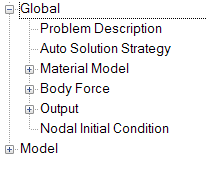
 on the toolbar to open the
Launch AcuSolve dialog.
on the toolbar to open the
Launch AcuSolve dialog.
 on the toolbar.
 on the toolbar in order to
properly display the plot.
on the toolbar in order to
properly display the plot.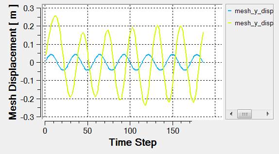
 icon on the toolbar.
 icon to turn off the outline
display.
Your model should now look like this:
icon to turn off the outline
display.
Your model should now look like this: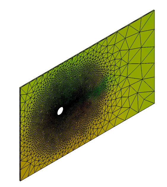
 to open the Boundary
Surface dialog.
to open the Boundary
Surface dialog.
 to open
the Coordinate Surface dialog.
to open
the Coordinate Surface dialog.