ACU-T: 5400 Piezoelectric Flow Energy Harvester: A Fluid-Structure Interaction (P-FSI)
This tutorial provides the instructions for setting up, solving, and viewing results for a simulation of a piezoelectric fluid harvester. In this simulation, a piezoelectric flow harvester is placed in a fluid flow channel. The harvester is attached to a cylinder mount which also acts as a bluff body causing vortices in the fluid flow. The interaction between the pressure fields generated by the vortices and the flow harvester structure is simulated in this tutorial. AcuSolve is used in conjunction with a structural solver to compute the structural displacement of the harvester using a practical fluid structure interaction (P-FSI) approach. Arbitrary Lagrangian Eulerian (ALE) approach is used to compute the mesh deformation in the fluid domain as it interacts with the deforming structure.
- Set up a Practical FSI simulation (P-FSI)
- Using ALE mesh motion
- Use Eigenmode Manager for transferring structural data onto CFD mesh
- Analyze the problem
- Start AcuConsole and create a simulation database
- Set general problem parameters
- Import the geometry for the simulation
- Create a volume group and apply volume parameters
- Create surface groups and apply surface parameters
- Set global and local meshing parameters
- Generate the mesh
- Set solution strategy parameters
- Import and transfer structural data onto the CFD mesh
- Set up the P-FSI simulation
- Set the appropriate boundary conditions
- Run AcuSolve
- Monitor the solution with AcuProbe
- Post-process the nodal output with AcuFieldView
Prerequisites
You should have already run through the introductory tutorial, ACU-T: 2000 Turbulent Flow in a Mixing Elbow. It is assumed that you have some familiarity with AcuConsole, AcuSolve, and AcuFieldView. You will also need access to a licensed version of AcuSolve.
Prior to running through this tutorial, copy AcuConsole_tutorial_inputs.zip from <Altair_installation_directory>\hwcfdsolvers\acusolve\win64\model_files\tutorials\AcuSolve to a local directory. Extract the files fluid.x_t and beam_modal.op2 from AcuConsole_tutorial_inputs.zip. The file fluid.x_t stores the geometry information for the fluid portion of the model for this problem, and the file beam_modal.op2 stores the output data from the structural solver which will be projected on to the CFD mesh that will be generated in the course of the tutorial.
The color of objects shown in the modeling window in this tutorial and those displayed on your screen may differ. The default color scheme in AcuConsole is "random," in which colors are randomly assigned to groups as they are created. In addition, this tutorial was developed on Windows. If you are running this tutorial on a different operating system, you may notice a slight difference between the images displayed on your screen and the images shown in the tutorial.
Analyze the Problem
An important step in any CFD simulation is to examine the engineering problem and determine the important parameters that need to be provided to AcuSolve. Parameters can be based on geometrical elements, such as inlets, outlets or walls, and on flow conditions, such as fluid properties, velocity or whether the flow should be modeled as turbulent or as laminar.
The system being simulated contains a section of a cantilever beam, the fixed side of which is attached to a rigid cylindrical body. The beam along with the cylinder is placed in a water flow stream. This cylindrical body acts a bluff body placed in the flow and stimulates vortex shedding in the flow downstream as it passes over the cylinder. The alternating shedding of vortices creates a zone of alternating asymmetric pressure distribution on either side of the beam. Such an alternating pressure distribution exerts an oscillating force on the beam, creating a sustainable oscillating vibration in the beam.
The modeled system can be compared to a piezoelectric based fluid flow energy harvester. The beam used in the structural model has a layered arrangement, with a brass shim sandwiched between the piezoelectric layers on either side. Piezoelectric materials have a unique property of generating an electric charge when subjected to stress. In the current arrangement as the fluid flow exerts an oscillating force on the beam leading to vibration, a corresponding oscillating structural stress is induced in the beam. The piezoelectric property comes into play here as the stress causes the piezoelectric layers to develop an electric charge. This electric charge is then tapped by a separate electromechanical arrangement. Thus there is a two-step energy conversion involved in this electricity generation process. First, the fluid flow energy is converted into mechanical energy of the vibration of the beam, then this mechanical energy is converted into electrical energy. However, the FSI aspect of this conversion, which is also of interest, is the transfer of energy between the fluid flow and beam.

Figure 1. Schematic of the Problem

Figure 2. The Beam with its Various Layers
Introduction to Theory
Fluid Structure Interaction
Fluid Structure Interaction is the interaction between a fluid flow and a deformable solid structure in contact with this flow. An FSI problem can be an external or an internal flow problem. The fluid flow can be external with the solid body immersed in the flow, for example, a windmill blade in open atmosphere. The fluid flow can also be internal with the solid body enclosing the flow, for example, fluid flow inside a deformable pipe. In both cases, the principle behind solving the problem remains the same. When a fluid flow encounters a structure, fluid pressure exerts a stress on the solid body that can lead to deformations in the structure. The magnitude of the deformation depends on the stiffness of the structure material and the magnitude of pressure force exerted by the fluid. The deformation in the structure shape then leads to altering of the flow characteristics in vicinity of the structure.
- Practical-FSI (P-FSI): The structure is reduced in the modal space and coupled to the fluid domain through interface nodes. The coupling between the solvers happens in a single pass itself. Structural behaviour is limited to be linear in a P-FSI simulation.
- Direct coupling (DC-FSI): The coupling is a co-simulation between the structural and the fluid solver, with each solver stepping through time simultaneously and iterating to equilibrium in each time step.
In case the deformations in the structure are large enough to alter the fluid flow significantly, the DC-FSI co-simulation approach should be used. With this approach, as the fluid flow and pressure fields affect the structural deformations, and the structural deformations affect the flow and pressure, the information about these effects is exchanged between the solvers in real time.
Given the difference in coupling methodology, it is likely that slightly different results will be observed when a same problem is solved using P-FSI and DC-FSI approaches. The choice of the approach that should be used shall depend on the problem and the available resources. As mentioned above, the P-FSI approach should be limited to the cases when displacements in the structure are small, and the structural behaviour can be approximated to be linear. For all other cases, DC-FSI should be preferred. However, DC-FSI simulations incur a higher computational resources cost. With this consideration, P-FSI simulation can also be used as a preliminary test simulation before a DC-FSI simulation is carried out.
FSI can be stable or oscillatory. In a stable FSI, the deformed shape of the structure will not change with time, unless the flow changes as well. In an oscillatory FSI, once the structure is deformed, it will try to return to its non-deformed state and then the whole deformation process repeats itself.
Mesh Motion Approaches in AcuSolve
Many simulations require deformation of the domain with time. AcuSolve provides two approaches for handling dynamic meshes:
- Arbitrary Lagrangian Eulerian (ALE)
- Interpolated Mesh Motion
This tutorial uses the ALE approach for specifying the mesh motion of the deformed nodes in the domain. The Interpolated Mesh Motion approach is discussed in detail in the subsequent tutorials which solve the same problem using this approach.
Arbitrary Lagrangian Eulerian (ALE)
ALE is an approach for mesh motion in which the computational nodes are moved arbitrarily with the aim of optimizing the element quality. An additional Partial Differential Equation (PDE) is solved to arrive at the appropriate mesh position. ALE is capable of handling complex arbitrary motions and is therefore the most general approach in simulating moving mesh problems. Generality comes with additional computational cost because of the extra PDE to be solved. For simpler motions like 1D or 2D motions faster approaches are available which include Interpolated Mesh Motion, general specified motions, Nodal Boundary conditions based approaches.
Define the Simulation Parameters
Start AcuConsole and Create the Simulation Database
In this tutorial, you will begin by creating a database, populating the geometry-independent settings, loading the geometry, creating volume and surface groups, setting group parameters, adding geometry components to groups, and assigning mesh controls and boundary conditions to the groups. Next you will generate a mesh and run AcuSolve to solve for the number of time steps specified. Finally, you will visualize some characteristics of the results using AcuFieldView.
In the next steps you will start AcuConsole and create the database for storage for the simulation settings.
-
Click the File menu, then click
New to open the New data
base dialog.
Note: You can also open the New data base dialog by clicking
 on the toolbar.
Set General Simulation Parameters
In next steps you will set parameters that apply globally to the simulation. To make this simple, the basic settings applicable for any simulation can be filtered using the BAS filter in the Data Tree Manager. This filter enables display of only a small subset of the available items in the Data Tree and makes navigation of the entries easier.
-
Click BAS in the Data Tree Manager to switch to basic view in the Data Tree.
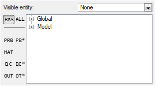
Figure 3. -
Change the Mesh type from Fixed to Arbitrary Mesh Movement
(ALE).
ALE stands for Arbitrary Lagrangian Eulerian. Using an ALE mesh type allows the mesh in the domain to be moved freely in accordance with the movement in the domain boundaries or interfaces. This is achieved by a formulation that can switch to purely Eulerian or purely Lagrangian or any arbitrary combination of the two thus allowing the elements to take the most optimum shape. This in turn enables the solver to handle a higher degree of element deformation.
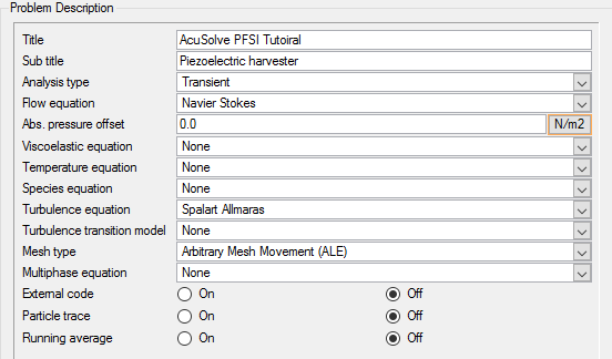
Figure 4.
Set Solution Strategy Parameters
In the next steps you will set parameters that control the behavior of AcuSolve as it progresses during the solution.
-
Make sure that Flow, Mesh and Turbulence are set to On.
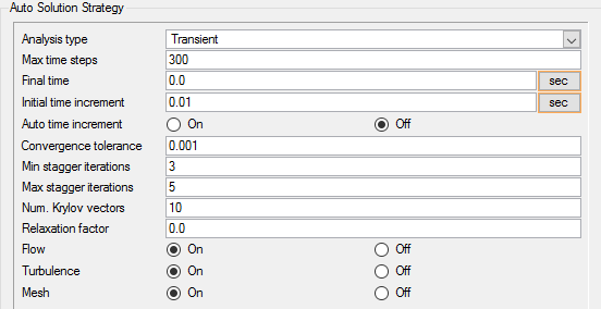
Figure 5.
Set Material Model Parameters
-
Double-click Material Model
in the Data Tree to expand it.
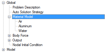
Figure 6. -
Save the database to create a backup
of your settings. This can be achieved with any of the following
methods.
- Click the File menu, then click Save.
- Click
 on
the toolbar.
on
the toolbar. - Click Ctrl+S.
Note: Changes made in AcuConsole are saved into the database file (.acs) as they are made. A save operation copies the database to a backup file, which can be used to reload the database from that saved state in the event that you do not want to commit future changes.
Import the Geometry and Define the Model
Import the Geometry
-
Select fluid.x_t and click
Open to open the Import Geometry
dialog.
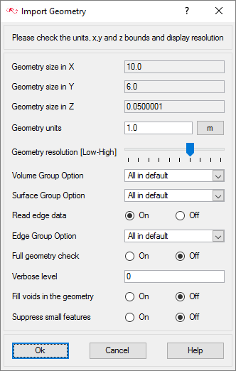
Figure 7.For this tutorial, the default values for the Import Geometry dialog are used to load the geometry. If you have previously used AcuConsole, be sure that any settings that you might have altered are manually changed to match the default values shown in the figure. With the default settings, volumes from the CAD model are added to a default volume group. Surfaces from the CAD model are added to a default surface group. You will work with groups later in this tutorial to create new groups, set flow parameters, add geometric components, and set meshing parameters.
-
Click Ok to complete
the geometry import.

Figure 8.
Apply Volume Parameters
Volume groups are containers used for storing information about a volume region. This information includes solution and meshing parameters applied to the volume and the geometric regions that these settings are applied to.
When the geometry was imported into AcuConsole, all volumes were placed into the "default" volume container. Since the model for this tutorial has only a single volume, it will be the only volume in the default volume group when the geometry is imported. Even when there is a single volume in the model, it is advisable to rename the volume for ease of identification in the future.
In the next steps you will rename the default volume group container and set the material and other properties for it.
-
Expand the Model tree item by clicking
 .
.
-
Expand Volumes. Toggle the display of the default
volume container by clicking
 and
and  next to the volume name.
Note: You may not see any change when toggling the display if Surfaces are being displayed, as surfaces and volumes may overlap.
next to the volume name.
Note: You may not see any change when toggling the display if Surfaces are being displayed, as surfaces and volumes may overlap. -
Set up the fluid volume element set.
-
Click the drop-down control next to Material model and select
Water.
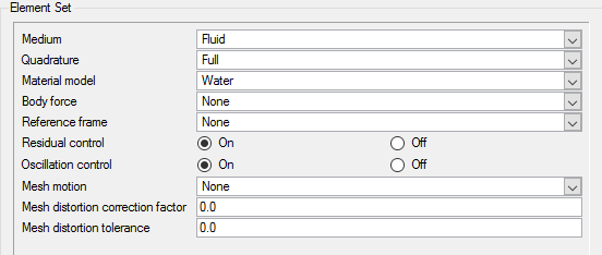
Figure 9.
-
Click the drop-down control next to Material model and select
Water.
Create Surface Groups and Apply Surface Parameters
Surface groups are containers used for storing information about a surface, including solution and meshing parameters, and the corresponding surface in the geometry that the parameters will apply to.
In the next steps you will define surface groups, assign the appropriate settings for the different characteristics of the problem, and add surfaces to the group containers.
In the process of setting up a simulation, you need to move into different panels for setting up the boundary conditions, mesh parameters, and so on, which can sometimes be cumbersome, especially for models with too many surfaces. To make it easier, less error prone, and to save time, two new dialogs are provided in AcuConsole. Use the Volume Manager and Surface Manager to verify and provide the information for all surface or volume entities at once. In this section some features of Surface Manager are exploited.
-
In the Surface Manager dialog, click New
six times to create six new surface groups.
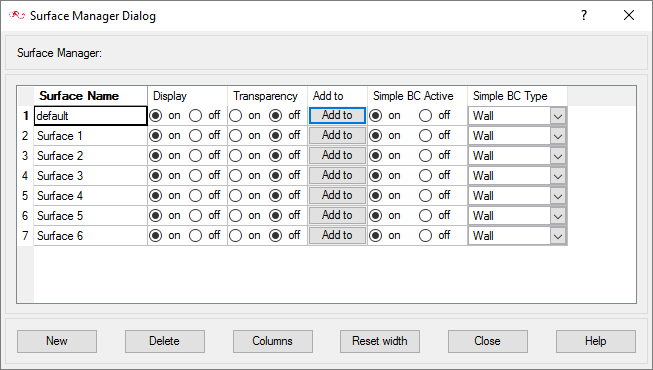
Figure 10.If you cannot see the Simple BC Active and Simple BC Type columns, click Columns , select these two columns from the list and click Ok.
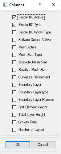
Figure 11. -
Set the Simple BC Active and Simple BC Type columns, per Figure 12.
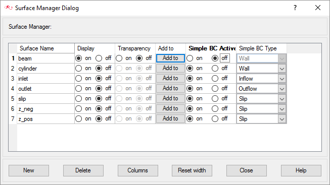
Figure 12. -
Assign the surfaces to the z_pos and z_neg surface groups.
-
Follow the procedure to assign the surface with the minimum
z-coordinate to the z_neg surface group.
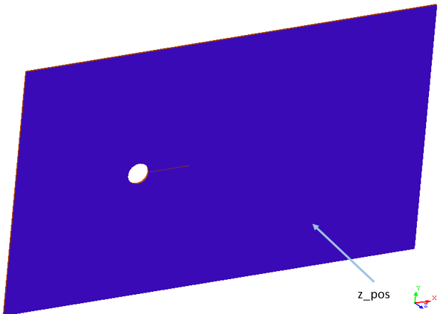
Figure 13.
-
Follow the procedure to assign the surface with the minimum
z-coordinate to the z_neg surface group.
-
Assign the cylinder surface to the cylinder surface group. This surface is the
contact boundary between the fluid and the cylinder. Use the following image as
the reference for selecting the required surfaces.
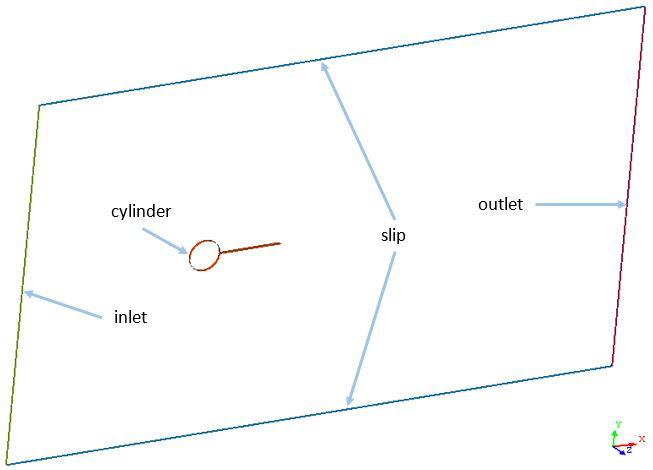
Figure 14.
When the geometry was loaded into AcuConsole, all geometry surfaces were placed in the default surface group container. This default surface group was renamed to beam in the Surface Manager. In the previous steps, you assigned some surfaces to various other surface groups that you created. At this point, all that is left in the beam surface group are the surfaces that make up the contact boundary between the fluid volume and the beam.
Create a Force Ramp Multiplier Function
The force acting on the beam due to the flow will be ramped gradually over the first few time steps. After these first few time steps the force on the beam will remain constant. This will be achieved using a multiplier function. In the next few steps you will create a linear multiplier function which will later be assigned as a force multiplier function for load acting on the beam.
-
Change the Curve fit variable to Time step.
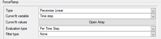
Figure 15. -
Fill in the values as follows:
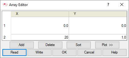
Figure 16.
Create a Flexible Body
In the introductory discussion of this tutorial, it was mentioned that FSI is the interaction between a fluid and a deformable, or in other words, flexible solid body. In AcuConsole, such a solid body is defined using the Flexible Body command. In P-FSI, the structure is reduced in the modal space. The Flexible Body definition includes the specification of mass, stiffness and damping matrices of the body. The mass matrix is usually normalized to I (unity matrix), and stiffness matrix k is a diagonal matrix where the diagonal entries each represent an Eigen value. The surface outputs list refers to the surfaces outputs which are used to calculate the forces and moments on the solid body.
-
Select beam as the entity in the row from the pull-down
menu.
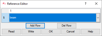
Figure 17. -
Click OK to close the dialog.
This tells the solver to use the surface output data on the beam surface group to determine forces to be transferred to the flexible body beam.
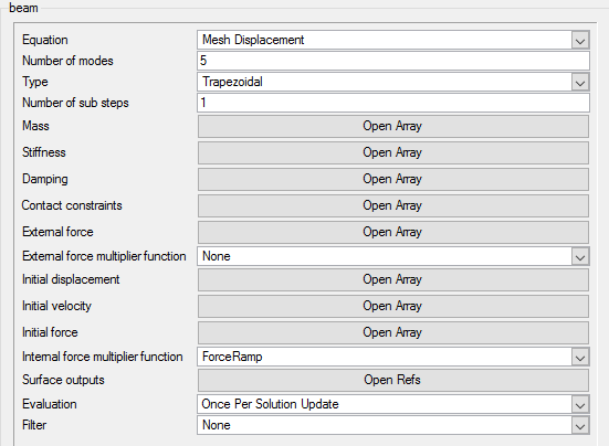
Figure 18.
Set Surface Boundary Conditions
Set Parameters for the Inlet
-
Set the Eddy viscosity to 1e-05 m2/sec.
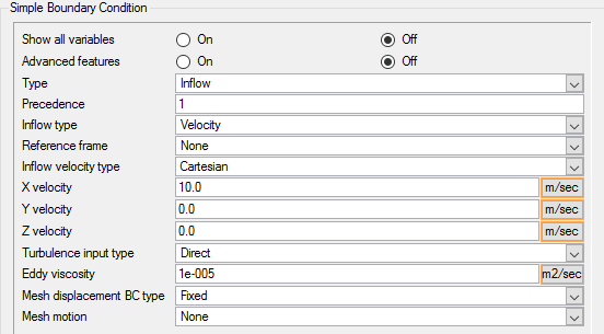
Figure 19.
Set Parameters for the z_neg and z_pos Surfaces
-
Set the Mesh displacement BC type to Slip
This setting allows the mesh to slip tangentially along the surface. Using this option requires the surface to be planar.
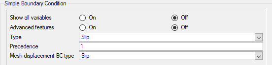
Figure 20. -
Repeat the above steps for the surface group z_pos.
You can also choose to Propagate the settings for z_neg surface group to z_pos surface group to ensure they are the same. To do this, right-click the Simple Boundary Condition entity under the z_neg surface group, select Propagate, select the z_pos surface group in the Propagate dialog and click Propagate to finish the propagation step.
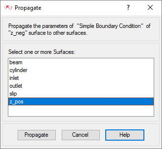
Figure 21.
Set Parameters for the Slip Surface
-
Ensure that the Type is set to Slip.
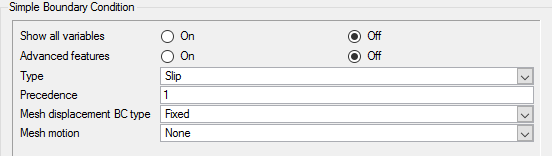
Figure 22.
Set Parameters for the Outlet Surface
-
Ensure that the Type is set to Outflow.
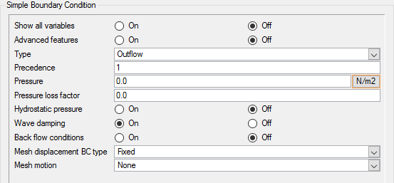
Figure 23.
Set Parameters for the Cylinder Surface
-
Ensure that the Type is set to Wall.
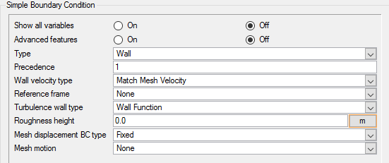
Figure 24.
Set Parameters for the Beam Surface
-
Set the Flexible body as the beam.
This instructs the solver to use the flexible body beam as the reference for calculating the mesh displacement of the beam surface group.
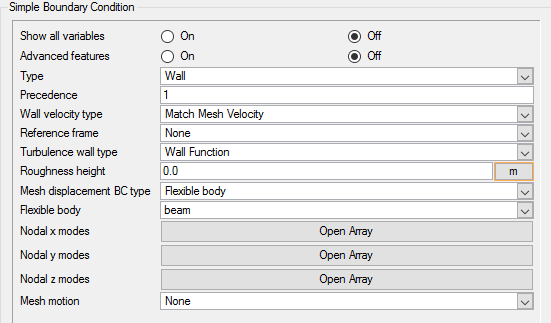
Figure 25.
Define Nodal Outputs
The nodal output command specifies the nodal output parameters, for example, output frequency and number of saved states.
-
Make sure that the Number of saved states is set to
0.
Setting this option to zero will instruct the solver to save all of the solution state files.
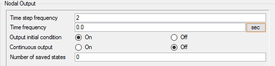
Figure 26.
Create Time History Output Points
-
Click Open Array next to the Coordinates option and fill
in the row in the Array Editor dialog as follows:
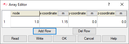
Figure 27. -
In the detail panel, set Time step frequency to 1.
This will save the results for the defined time history point at every time step.
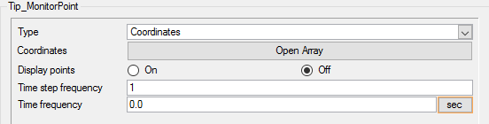
Figure 28.
Set Initial Conditions
-
Set the Eddy viscosity to 1e-05 m2/sec.
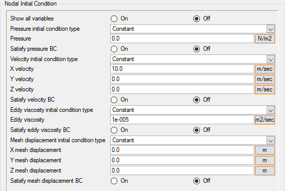
Figure 29.
Assign Mesh Controls
Set Global Mesh Parameters
Global mesh attributes are the meshing parameters applied to the model as a whole without reference to a specific geometric volume, surface, edge or point. Local mesh attributes are used to create mesh generation controls for specific geometry components of the model.
In the next steps you will set the global mesh attributes.
-
Set the Mesh growth rate to 1.4.
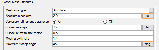
Figure 30.
Set Surface Mesh Parameters
Surface mesh attributes are applied to a specific surface in the model. It is a type of local meshing parameter used to create targeted mesh controls for one or more specific surfaces.
Surface mesh attributes are applied to a specific surface in the model. It is a type of local meshing parameter used to create targeted mesh controls for one or more specific surfaces.
Setting local mesh attributes, such as surface mesh attributes, is not mandatory. When a local mesh attribute is not found for a component, the global attributes are used as the mesh generation control for that component. If a local mesh attribute is present, it will take precedence over the global setting.
In the next steps you will set the surface meshing attributes.
-
Set the remaining settings as follows:
-
Set the Boundary layer elements type to
Tetrahedron.
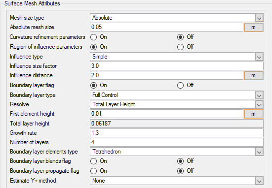
Figure 31.
-
Set the Boundary layer elements type to
Tetrahedron.
-
Click the beam surface group in the
Propagate dialog.
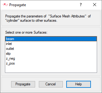
Figure 32.
Define Mesh Extrusion
The present simulation is equivalent to a representation of a 2D cross section of the model. In AcuSolve, 2D models are simulated by having just one element across the faces of the cross section. When these faces are set up with a similar boundary condition it coerces the corresponding nodes across the faces to have the same results. In this problem these faces are the negative and positive z-surfaces. This kind of mesh is achieved in AcuSolve with mesh extrusion process. In the following steps, the process of extrusion of the mesh between these surfaces is defined.
-
In the Mesh Extrusion dialog, make the following
settings.
- Check that the Geometry type is set to surface.
- Use the drop-down arrows to select the surfaces for Side 1 and Side 2 as z_neg and z_pos, respectively.
- Check that the Extrusion type is set to Number of layers.
- Set Number of layers to 1.
- Set Extrusion options to Mixed Elements.
Use the following image for reference for setting up the mesh extrusion.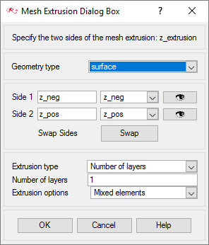
Figure 33.
Generate the Mesh
In the next steps you will generate the mesh that will be used when computing a solution for the problem.
-
Click
 on the toolbar to open the Launch
AcuMeshSim dialog.
For this case, the default settings will be used.
on the toolbar to open the Launch
AcuMeshSim dialog.
For this case, the default settings will be used. -
Click Ok to begin meshing.
During meshing an AcuTail window opens. Meshing progress is reported in this window. A summary of the meshing process indicates that the mesh has been generated.
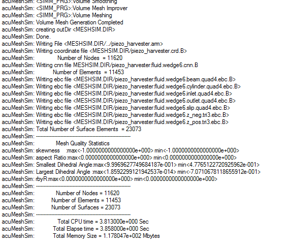
Figure 34.Note: The actual number of nodes, elements and memory usage may vary slightly from machine to machine.
Import Structural Model Information
-
Click
 on the
toolbar.
The Eigenmode Manager dialog opens.
on the
toolbar.
The Eigenmode Manager dialog opens. -
Type Modes as the Name for the entry.
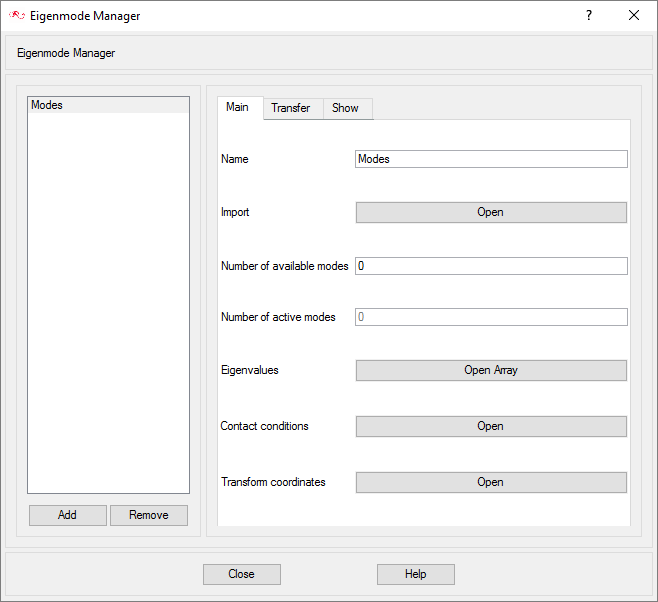
Figure 35. -
Click Transfer next to the Flexible body option.
-
Make sure that beam is selected in the Reference
Editor dialog that opens.
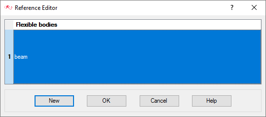
Figure 36.
-
Make sure that beam is selected in the Reference
Editor dialog that opens.
-
Click Transfer next to the Simple BC option.
-
Select beam from the list in the
Reference Editor dialog.
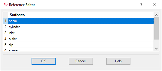
Figure 37.
-
Select beam from the list in the
Reference Editor dialog.
Compute the Solution and Review the Results
Run AcuSolve
In the next steps you will run AcuSolve to compute the solution for this case.
-
Click
 on the toolbar to open the
Launch AcuSolve dialog.
For this case the default settings will be used. AcuSolve will run using four processors, if available, a higher number of processors may be specified. AcuConsole will generate AcuSolve input files and will launch AcuSolve. AcuSolve will calculate the transient solution for this problem.
on the toolbar to open the
Launch AcuSolve dialog.
For this case the default settings will be used. AcuSolve will run using four processors, if available, a higher number of processors may be specified. AcuConsole will generate AcuSolve input files and will launch AcuSolve. AcuSolve will calculate the transient solution for this problem. -
Click Ok to start the solution process.
While computing the solution, an AcuTail window opens. Solution progress is reported in this window. A summary of the solution process indicates that the run has been completed.
The information provided in the summary is based on the number of processors used by AcuSolve. If you use a different number of processors than indicated in this tutorial, the summary for your run may be slightly different than the summary shown.
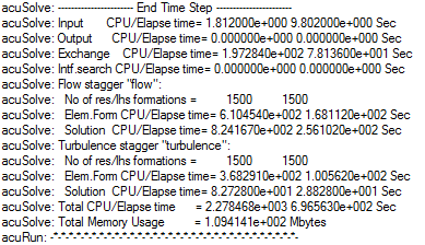
Figure 38.
Post-Process with AcuProbe
AcuProbe can be used to monitor various variables over solution time.
-
Open AcuProbe by clicking
 on the toolbar.
-
Right-click on mesh_y_displacement and select
Plot.
Note: You might need to click
 on the toolbar in order to
properly display the plot.
on the toolbar in order to
properly display the plot.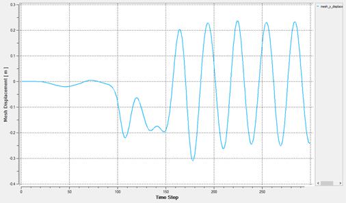
Figure 39.The node 1 lies at the tip of the beam. The plot above shows the displacement of the tip of the beam due to the fluid forces as the beam interacts with the flow.
Post-Process with AcuFieldView
- How to find the data readers in the File menu and open up the desired reader panel for data input.
- How to find the visualization panels either from the Side toolbar or the Visualization panel on the Main menu to create and modify surfaces in AcuFieldView.
- How to move the data around the modeling window using
mouse actions to translate, rotate and zoom in to the data.
This tutorial shows you how to work with steady state analysis data.
Start AcuFieldView
-
Click
 on the
AcuConsole toolbar to open the
Launch AcuFieldView dialog.
on the
AcuConsole toolbar to open the
Launch AcuFieldView dialog.
-
Click Ok in the Launch AcuFieldView dialog.
You will see that the pressure contours have already been displayed on all of the boundary surfaces with mesh. When results of a transient simulation are loaded in AcuConsole the displayed results correspond to the last time step of the simulation.
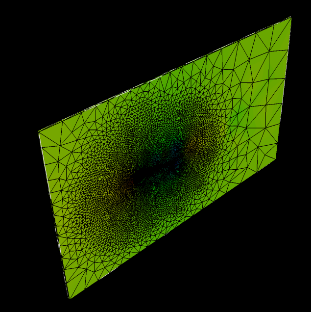
Figure 40.
Set Up AcuFieldView
-
Click Viewer Options.
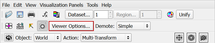
Figure 41. -
In the Viewer Options dialog:
-
Disable the axis markers by clicking Axis
Markers.
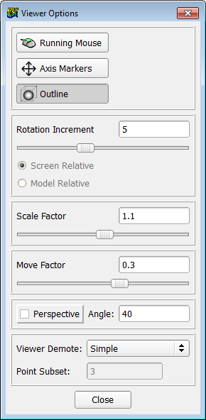
Figure 42.
-
Disable the axis markers by clicking Axis
Markers.
-
Click the
 icon on the toolbar.
-
Click Background in the Scalar Colormap
Specification dialog.
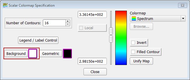
Figure 43. -
Select the color white in the Background Color
dialog.
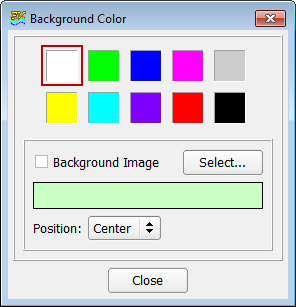
Figure 44. -
Click the
 icon to turn off the outline
display.
Your model should now look like this:
icon to turn off the outline
display.
Your model should now look like this: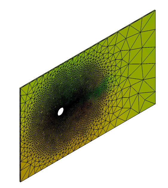
Figure 45.
Visualize and Save an Animation of the Beam Displacement
-
Click
 to open the Boundary
Surface dialog.
to open the Boundary
Surface dialog.
-
Click
 to open
the Coordinate Surface dialog.
to open
the Coordinate Surface dialog.
-
From the Defined Views menu bar, select +Z as the
viewing direction.
Your model should look like the image below. The visible shape of the beam is its deformed shape at the end of last time step in the simulation.
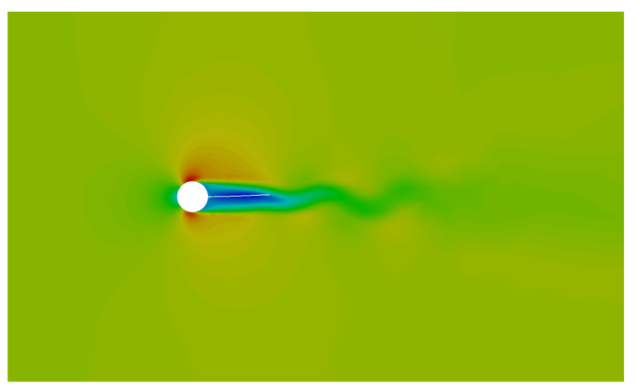
Figure 46. -
Click .
The Transient Data Controls dialog opens.
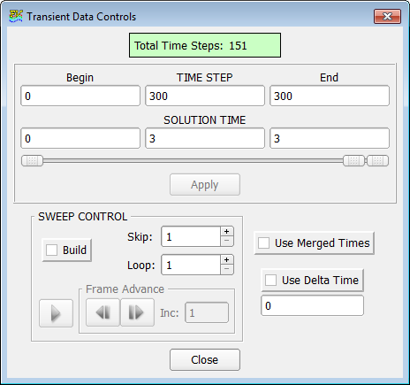
Figure 47.If the Sweep Control in this dialog shows Sweep instead of Build, the Flipbook Build Mode is not active. In Sweep mode, you will be able to create and visualize the animation but you will not be able to save it. To be able to save the animation, enable the Flipbook Build Mode.
-
Click Apply.
The displayed state now corresponds to the initial state of the domain.
Figure 48. -
Click the
 icon to play the animation.
As the animation progresses, you will be able to see the alternating vortices on the top and bottom surface of the beam, causing an oscillating motion in the beam. This oscillating motion is responsible for generation of piezoelectric charge in the top and bottom layers of the beam.
icon to play the animation.
As the animation progresses, you will be able to see the alternating vortices on the top and bottom surface of the beam, causing an oscillating motion in the beam. This oscillating motion is responsible for generation of piezoelectric charge in the top and bottom layers of the beam. -
To save the animation click the
 icon and then click Save.
Summary
In this AcuSolve tutorial you successfully set up and solved a FSI problem using the Practical-FSI or P-FSI approach. The modal analysis of the structure (beam) is first done in a structural solver and the results of this modal analysis are used to represent the structure in AcuConsole. The results of the modal analysis provide the necessary information, such as the mass, stiffness and damping characteristics of the solid body, to AcuSolve. This information, along with the flow field information generated by AcuSolve, is used to calculate the displacement of the beam as it interacts with the flow.
You started the tutorial by creating a database in AcuConsole, importing and meshing the fluid portion geometry and setting up the basic simulation parameters. Then you set up a flexible body to represent the beam and generated a solution with AcuSolve.
Results were post-processed in AcuFieldView where you generated an animation of the beam’s displacement as it interacts with the fluid flow. New features that were introduced in this tutorial include setting up a Practical FSI simulation (P-FSI), using ALE mesh motion and using Eigenmode Manager in AcuConsole for transferring structural data onto a CFD mesh.