This tutorial provides the instructions for setting up, solving and viewing
results for a simulation of flow around a static ship hull. In this
simulation, a wave hits the static ship hull and the flow around the ship is
simulated. This tutorial is designed to introduce you to a number of
modelling concepts necessary to perform Free-Surface simulations.
The basic steps in any CFD simulation are shown in ACU-T: 2000 Turbulent Flow in a Mixing Elbow. The following additional
capabilities of AcuSolve are introduced in this
tutorial:
Use of a User Defined Function (UDF) for the gravity wave
generation
Mesh extrusions
Periodic boundary conditions
Use of Surface Manager to apply surface
attributes
Free surface
Guide surface
Use of hydrostatic pressure for boundary conditions
Arbitrary mesh motion using ALE (Arbitrary Lagrangian-Eulerian)
method
In this tutorial you will do the following:
Analyze the problem
Start AcuConsole and create a
simulation database
Set general problem parameters
Set solution strategy parameters
Import the geometry for the Wigley-hull
Create a volume group and apply volume parameters
Create surface groups and apply surface parameters
Set global meshing parameters
Set mesh extrusion and periodic boundary conditions
Generate the mesh
Run AcuSolve
Monitor the solution with AcuProbe
Post-processing the nodal output with AcuFieldView
Prerequisites
You should have already run through the introductory tutorial, ACU-T: 2000 Turbulent Flow in a Mixing Elbow. It is assumed that you have some
familiarity with AcuConsole, AcuSolve, and AcuFieldView. You will
also need access to a licensed version of AcuSolve.
Prior to running through this tutorial, copy
AcuConsole_tutorial_inputs.zip from
<Altair_installation_directory>\hwcfdsolvers\acusolve\win64\model_files\tutorials\AcuSolve
to a local directory. Extractwigley_hull.x_t and
wave.cfrom AcuConsole_tutorial_inputs.zip.
The color of objects shown in the modeling window in this tutorial and those displayed on your screen may differ. The default color
scheme in AcuConsole is "random," in which colors are
randomly assigned to groups as they are created. In addition, this tutorial was
developed on Windows. If you are running this tutorial on a different operating system,
you may notice a slight difference between the images displayed on your screen and the
images shown in the tutorial.
Analyze the Problem
The problem to be addressed in this tutorial is shown in Figure 1. It is a mid-section of a
Wigley Ship model. Wigley hulls have been widely used as test cases for evaluating
hydrodynamic behavior of ships. The present tutorial demonstrates the simulation of gravity
waves hitting a static Wigley hull (a hypothetical situation of a ship anchored in sea).
Since the motion considered in this tutorial is perpendicular to the length of the ship, an
analysis of a 2D section of the ship hull would be appropriate with lesser computation time
without compromising on accuracy. The mid-section dimensions of the Wigley hull is a
function of total ship length and the model used in this tutorial is the mid-section of
Wigley hull whose ship length is 1 m. Figure 1. Schematic of a Ship Hull
Generation of Surface Gravity Waves
Gravity waves are waves generated in a fluid medium or at the interface between two media
when the force of gravity or buoyancy tries to restore equilibrium. An example of such an
interface is that between the atmosphere and the ocean, which gives rise to wind waves
[1]. The mechanism of surface gravity waves is that a fluctuation causes water
to rise above the equilibrium surface level, gravity pulls it back down because water is
heavier than air, inertia acquired during the falling movement causes water to penetrate
below its level of equilibrium and a bouncing motion results. The oscillation is similar to
that of a spring that has been stretched and released. The ‘spring’ action in a surface
water wave is the gravity, hence the name of surface gravity wave [2]. In the
present simulation, wind-generated gravity waves on the free surface of the sea are
generated using a UDF (User-Defined Function). Figure 2. Gravity Waves
Figure 2 depicts parameters that define a simple,
progressive gravity wave. This wave can be modeled in the form of the sinusoidal wave
profile, shown below.
(1)
where
is the horizontal particle velocity of wave
is the speed of the wave
U is the velocity amplitude of disturbance
is wave number =
is the wave length of the wave
is the depth of the water
is the frequency of the wave =
is the time period of the wave
t is the time
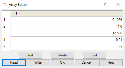
In the present simulation we use the following values for the variables of above
equation:
U = 0.1256 m/s
= 1.0 sec
= 12.566 m-1
= 0.01 m/s
= 0.5 m
In the present tutorial, at the inlet you will generate the wave for 2 seconds and simulate
the motion of the wave for 5 seconds. A UDF (wave.c) written in C language is used for this
purpose. For the details of the functions used in the wave.c, refer to the AcuSolve
User-Defined Functions Manual.
Two Dimensional Simulations in AcuSolve
AcuSolve does not support a CFD analysis on a 2D surface mesh. However a
2D analysis can be simulated on a volume mesh by having a single element extrusion along the
perpendicular direction of 2D surface of interest and then having identical boundary
conditions of symmetry or slip on both sides of extrusion. This way you can ensure that the
solution does not vary along the thickness (extrusion), which is essentially a 2D
representation of the problem. The present tutorial uses this approach.
Define the Simulation Parameters
Start AcuConsole and Create the Simulation Database
In this tutorial, you will begin by creating a database, populating the
geometry-independent settings, loading the geometry, creating groups, setting group
attributes, adding geometry components to groups, and assigning mesh controls and
boundary conditions to the groups. Next you will generate a mesh and run AcuSolve to solve for the number of time steps specified.
Finally, you will visualize some characteristics of the results using AcuFieldView.
Start AcuConsole from the Windows Start menu by clicking Start > Altair <version> > AcuConsole.
Click the File menu, then click
New to open the New data
base dialog.
Note:You can also open the
New data base dialog by clicking on the toolbar.
Browse to the location that you would like to use as your working
directory.
This directory is where all files related to the simulation will
be stored. The AcuConsole database file
(.acs) is stored in
this directory. Once the mesh and solution are created, additional files and
directories will be created within this directory.
Create a new directory in this location. Name it
Ship_hull_static and open this directory.
Enter Ship_hull_static as the file name for the
database, or choose any name of your preference.
Note: In order for other applications to be able to read the
files written by AcuConsole, the database
path and name should not include spaces.
Click Save to create the database.
Set General Simulation Parameters
In next steps you will set attributes that apply globally to the simulation.
To simplify this task, you will use the BAS filter in the Data Tree Manager. This filter reduces the number of items shown in
the Data Tree to make navigation of the entries easier.
The general attributes that you will set for this tutorial are for turbulent flow,
transient analysis, and mesh type as arbitrary mesh movement (ALE).
Click BAS in the Data Tree Manager to switch to basic view in the Data Tree.
Figure 3.
Expand the GlobalData Tree item.
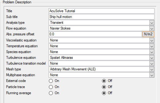
Double-click Problem
Description to open the Problem
Description detail panel.
Enter AcuSolve Tutorial as the Title for this
case.
Enter Ship hull motion as the Sub title for this
case.
Click the Analysis type drop down menu and select
Transient.
Change the Turbulence equation to Spalart
Allmaras.
Set the Mesh type to Arbitrary Mesh Movement
(ALE).
Figure 4.
Set Solution Strategy Attributes
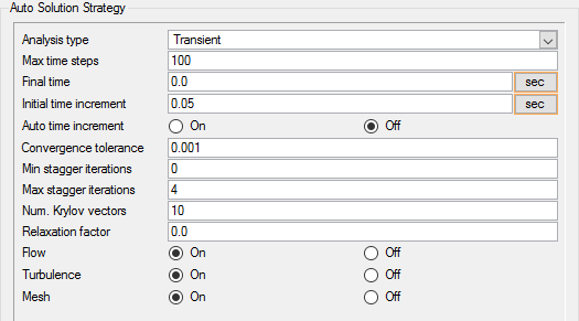
Double-click Auto Solution
Strategy to open the Auto Solution
Strategy detail panel.
Ensure the Analysis type is set to Transient.
Set the Max time steps to 100.
Set the Initial time increment to 0.05 seconds.
Change the Max stagger iterations to 4.
Stagger iterations define how many iterations will be performed within each
time step. Changing the maximum stagger iterations to 4 means that AcuSolve will perform a maximum of four iterations at every time
step whether convergence is achieved or not. Setting the minimum stagger
iterations to 0 indicates that there is no minimum number of iterations within a
time step. In this case, AcuSolve will proceed to the next
time step when it has either reached the desired convergence tolerance or the
maximum number of stagger iterations within the step.
Check that the Relaxation factor is set to 0.0.
When solving transient solutions, the relaxation factor should be set to zero.
A non-zero relaxation factor causes incremental updates of the solution, which
will impact the time accuracy of the solution for transient cases. Figure 5.
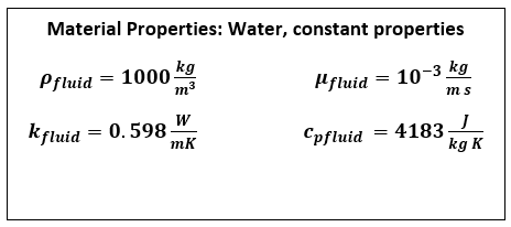
Set Material Model Parameters
AcuConsole has three pre-defined materials, Air,
Aluminum and Water, with standard parameters defined. In the next steps you will check
the material properties of the predefined Water to match the desired properties for this
problem. Figure 6.
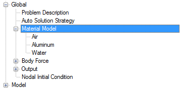
Double-click Material Model
in the Data Tree to expand it.
Figure 7.
Double-click Water in the
Data Tree to open the Water
detail panel.
The material type water air is Fluid. Fluid
is the default material type for any new material created in AcuConsole.
Click the Density tab. The density of water is 1000.0
kg/m3.
Click the Viscosity tab. The viscosity of water is 0.001
kg/m – sec.
Save the database to create a backup
of your settings. This can be achieved with any of the following
methods.
Click the File menu, then click
Save.
Click on
the toolbar.
Click Ctrl+S.
Note: Changes made in AcuConsole are saved into
the database file (.acs) as they are made. A save operation copies the database to
a backup file, which can be used to reload the database from that saved
state in the event that you do not want to commit future changes.
Import the Geometry and Define the Model
Import the Geometry
You will import the geometry in the next
part of this tutorial. You will need to know the location ofwigley_hull.x_tin order to complete these steps. This file contains
information about the geometry in ParasolidASCII format.
Click File > Import.
Browse to the directory containing wigley_hull.x_t.
Change the file name filter to Parasolid File (*.x_t *.xmt *X_T
…).
Select wigley_hull.x_t and click
Open to open the Import Geometry
dialog.
Figure 8.
For this tutorial, the default values for the Import
Geometry dialog are used to load the geometry. If you have previously
used AcuConsole, be sure that any settings that you
might have altered are manually changed to match the default values shown in the
figure. With the default settings, volumes from the CAD model are added to a default
volume group. Surfaces from the CAD model are added to a default surface group. You
will work with groups later in this tutorial to create new groups, set flow
parameters, add geometric components, and set meshing parameters.
Click Ok to complete
the geometry import.
Figure 9.
Rotate the visualization to view the entire model.
Set Body Force
As discussed in the section Analyze the Problem, gravity is
the important aspect of the simulation. In AcuConsole it is
defined as the Body Force of standard Gravity (g = 9.81 m/s2) along the
Z-axis is applied to the model.
In the Data Tree, double-click Body
Force to expand it.
Double-click Gravity to open the detail panel.
The Medium for Gravity is Fluid. The Gravity defined here is applicable only
on material models whose material type is Fluid.
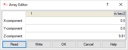
Next to the Gravity field, click Open Array.
In the X-components and Y-components fields, enter
0.
In the Z-components field, enter 9.81
m/s2
Click OK to complete the definition of Gravity.
Figure 10.
Note: The definition of Gravity here will have no effect on the simulation
unless it assigned to a Volume in the model.
Apply Volume Attributes
When the geometry was imported into AcuConsole, all volumes were placed into the "default" volume
container.
In the next steps you will rename the default volume group container, set the
material for that group and set mesh motion for the fluid volume.
Minimize Global in the Data Tree Manager and expand the Model
tree item by clicking .
Expand the Volumes tree item.
Expand Volumes. Toggle the display of the default
volume container by clicking
and next to the volume name.
Note: You may not see any change when toggling the display if
Surfaces are being displayed, as surfaces and
volumes may overlap.
Create a new volume group for the solid ship hull.
Right-click on Volumes.
Click New.
Rename the new volume group to Guide_Vol_Ship.
Add the ship hull component in the geometry to this group.
Right-click Guide_Vol_Ship.
Click Add to.
Click the ship hull portion of the geometry in the modeling window.
If you rotate the view by Ctrl+ left-clicking,
you can see that only the ship volume is highlighted. Figure 11.
Click Done to add the selected volume to the
solid volume group.
Set the medium for the volume to None.
The material model of the ship hull is inappropriate to the present
simulation. Hence, the medium is set to None.
Note: The element sets of the solid
volume are necessary in the pre-processing stage (AcuPrep) of the simulation for the evaluation of
normal directions for the guide surfaces. However the element sets are not
necessary during the solver module because the only interaction between the
fluid and solid is at the guide surface. The use of None for the Medium of
this volume ensures that no elements of this volume are carried over to the
solver, thus saving the computational time.
Expand the Guide_Vol_Ship volume group in the
tree.
Double-click Element Set to open the
Element Set detail panel.
Change the Medium to None.
Check that the Mesh motion is set to None.
When the geometry was loaded into AcuConsole,
all geometry volumes were placed in the default volume group container. In the
previous steps, you selected a geometry volume to be added to Guide_Vol_Ship
container that you created. At this point, all that is left in the default volume
group is the fluid volume. Rather than create a new container, add the fluid volume
in the geometry to it, and then delete the default volume container, you can rename
the container and modify the attributes for this group.
In the Data Tree, right-click on
default and rename it to
Fluid.
Set up the Fluid volume element set.
Expand the Fluid volume group in the tree.
Double click Element Set under Fluid to open it
in the detail panel.
Ensure that the Medium for the volume is set to Fluid. If not, change
it to Fluid.
Change the Material model to Water.
Change the Body force to Gravity.
Create Surface Groups and Apply Surface Parameters
Surface groups are containers used for storing information about
a surface, including solution and meshing parameters, and the corresponding surface
in the geometry that the parameters will apply to.
In the next steps you will define surface groups,
assign the appropriate settings for the different characteristics of the problem,
and add surfaces to the group containers.
In the process of setting up a simulation, you need to move into
different panels for setting up the boundary conditions, mesh parameters, and so on,
which can sometimes be cumbersome, especially for models with too many surfaces. To
make it easier, less error prone, and to save time, two new dialogs are provided in
AcuConsole. Use the Volume
Manager and Surface Manager to verify and
provide the information for all surface or volume entities at once. In this section
some features of Surface Manager are exploited.
Turn-off display for Volumes by right-clicking Volumes
and selecting Display off .
Right-click Surfaces in the Data Tree and select Surface
Manager.
In the Surface Manager dialog, click New
eight times to create eight new surface groups.
Turn off the display for all surfaces except for the default surface.
Rename the default surface to Hull_guide.
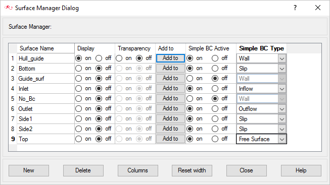
Rename Surface 1 through Surface 8 and set the Simple BC Type and Simple BC
Active options according to the figure below.
Figure 12.
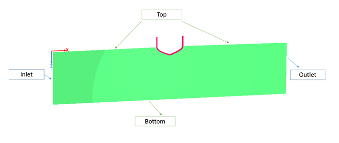
Assign the surface for Outlet.
In the Surface Manager, next to Outlet, click Add
to.
Select the surface of the Fluid with maximum X-coordinate.
Click Done.
Figure 13.
Similarly, add the following surface to the appropriate surface groups.
Bottom: Surface with maximum Z-coordinate (Bottom surface of water)
Top: Two surfaces at minimum Z-coordinate (Top surfaces of water)
Side1: Surface with maximum Y-Coordinate
Side2: Surface with minimum Y-Coordinate
Inlet: Surface with minimum X-Coordinate
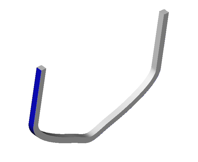
No_Bc: 5 surfaces of the Guide_Vol_Ship that are not in contact with
Fluid as shown below. Surfaces shown in gray belong to the No_Bc surface
set. Figure 14.
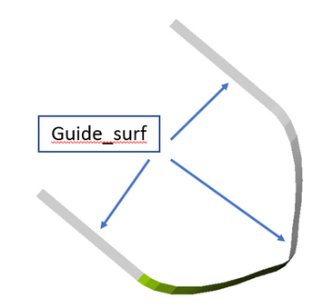
Assign the surface for Guide_surf.
Guide_surf is the surface that belongs to the Guide_Vol_ship and is in contact
with Fluid.
In the Surface Manager, next to Guide_surf, click Add
to.
Select all of the surfaces that belong to the Guide_vol_ship and are in
contact with Fluid.
Figure 15.
Assign the surface for Hull_guide.
Hull_guide is the surface that belongs to the fluid and is in contact with the
Guide_Vol_Ship. At this point, all the surfaces present in the default Surface
set are eligible for Hull_Guide.
In the Surface Manager, next to Hull_guide, click Add
to.
Select all of the surfaces present in the default surface set.
Figure 16.
Clear the empty surface sets.
In the Data Tree, right-click
Surfaces and select
Purge.
Make sure that all the surfaces in Hull_guide belong to Fluid Volume and all
surfaces in Guide_surf belong to Guide_Vol_ship Volume.
Under Surfaces, right-click Hull_guide and
select Info.
In the Information Window, check that Parent
Volume is Fluid.
Under Surfaces, right-click Guide_surf and
select info.
In the Information Window, check that Parent
Volume is Guide_Vol_ship for all the surfaces in Guide_surf.
Close the Surface Manager.
Side1 and Side2
The present simulation is a 2D representation of a ship in water. Hence it is
appropriate to set the Side1 and Side2 with the slip boundary condition to simulate
that effect.
In the Data Tree, expand
Side1.
Double-click Simple Boundary Condition to open the
Simple Boundary Condition detail panel.
Check that the Type is Slip.
Change the Mesh displacement BC type to Slip.
Repeat the settings for the surface Side2.
AcuConsole has a special feature named
Propagate that can speed up the process of simulation setup and
save time. This feature copies the attributes (it may be Simple Boundary Condition,
Surface Output, Surface Mesh Attributes, Element Set, Volume Mesh Attributes, and so
on) set for one surface set or volume set to another surface set or volume set. For
example, in a simulation model if there are 10 surface sets with simple boundary
condition set to Slip, then you can use this feature. You need to manually set the
boundary condition for one surface and use the Propagate feature for all other
surfaces.
Under Side1, right-click Simple Boundary Condition and
select Propagate.
Select the surface Side2 and click
Propagate.
Top
The Top surface is the top surface of water which is in contact with air and hence
Free Surface is the appropriate boundary condition.
Note: As the name suggest, the
free surface is a surface of the fluid which is not constrained by any physical
boundary. This type of the boundary condition imposes normal component of mesh
velocity to the flow velocity at this surface.
In the Data Tree, expand
Top.
Double-click Simple Boundary Condition to open the
Simple Boundary Condition detail panel.
Check that the Type is Free Surface.
Check that the Surface tension model is set to None.
Note: Surface tension model is the user-given model of surface tension defined
under Global > Surface Tension Model. Since the surface tension is not modelled in this
simulation, this parameter is set to None.
Check that the Contact angle model is set to None.
Note: Contact angle model is the user-given model of contact angle defined under Global > Contact Angle Model. The contact angle model is used in conjunction with the
surface tension model. Since the surface tension is not modelled in this
simulation, this parameter is set to None.
Check that the Pressure is set to 0.
Check that the Pressure loss factor is set to 0.
Note: Use of Pressure loss factor (k) would add the following term to the
pressure term
where
= -1 for the inflow
=1 for the outflow
k = Pressure loss factor
= density of fluid
u = velocity of
fluid
n = outward pointing normal of the
surface
The higher the value of pressure loss factor, stiffer the
free surface behaves, that is, lesser the displacement of the free
surface.
Bottom
In the Data Tree, expand
Bottom.
Double-click Simple Boundary Condition to open the
Simple Boundary Condition detail panel.
Check that the Type is Slip.
A simple boundary condition type Slip imposes zero nodal boundary condition on
velocity normal to the given surface.
Change the Mesh displacement BC type to Fixed.
The Bottom surface is a stationary surface and a Mesh displacement BC type
Fixed imposes zero mesh displacement with respect to the surface.
Outlet
In the Data Tree, expand
Outlet.
Double-click Simple Boundary Condition to open the
Simple Boundary Condition detail panel.
Check that the Type is Outflow.
Use the default values for Pressure and Pressure loss factor.
Change Hydrostatic pressure to On.
The pressure is not constant throughout the Outlet surface. The pressure at
this surface varies along Z- axis because of gravity (Hydrostatic pressure
variation). In general, when setting Hydrostatic pressure to On, the pressure
varies as given below
where
= density of fluid
z = coordinate vector of the point
on the surface
z0 = coordinate vector where the hydrostatic
pressure is zero. Z0 defined below using Hydrostatic pressure
origin
g = gravity vector
Next to Hydrostatic pressure origin, click Open Array to
define the pressure origin.
Provide the coordinates of origin (0, 0, 0) in the Array
Editor.
Note: Hydrostatic pressure will be zero on Free surface (that is, the Top
surface). The point (0, 0, 0) is on the Top surface. In particular, any
point on the Top surface can be chosen as Hydrostatic pressure
origin.
During the simulation there will be certain time points (particularly when
trough is formed at the outlet surface) at which the flow enters the domain through
certain portion of outlet surface, which is called back flow. Back flow may lead to
instability temperature, turbulence variables. Enabling Back flow conditions allows
nodal boundary conditions to be specified for these variables only on nodes where
there is flow re-entering the domain. Assuming the outlet is sufficiently far away
from ship hull, eddy viscosity value can set as that of the Inlet, for example,
1e-05
Set Back flow conditions to On.
Set the Eddy viscosity back flow type to Value.
Set Eddy viscosity to 1e-05.
Change the Mesh displacement BC type to Slip.
Setting the Mesh displacement BC type to Slip will allow the nodes on this
surface (Outlet) to move freely along the surface.
No_Bc
The No_Bc surface set contains the surfaces of Guide_Vol_Ship which do not
participate in actual simulation. Hence it is appropriate to disable the Boundary
condition for this surface.
In the Data Tree, expand
No_Bc.
Uncheck the Simple Boundary Condition check box.
Guide_surf
This surface belonging to the Guide_Vol_Ship will remain stationary in the present
simulation and provide as a guide for the fluid around. Hence we define it as Guide
Surface with no mesh motion.
In the Data Tree, expand
Guide_surf.
Uncheck the Simple Boundary Condition check box.
Note: This ensures that boundary condition for the Guide_surf surface is not
defined by using Simple Boundary Conditions. The boundary condition will be
defined as a Guide surface using the following steps.
Click ALL in the Data Tree Manager.
Under the Guide_Surf surface, check the box next to Guide Surface.
The Guide Surface type will ensure that Guide_Surf surface can be used to
guide mesh nodes of Hull_guide surface. Refer to the Hull_guide surface
attributes defined later in this tutorial.
Make sure that Mesh motion is set to None.
This ensures that the Guide_surf surface is static and has no
motion.
Hull_guide
In the Data Tree, expand
Hull_guide.
Double-click Simple Boundary Condition to open the
Simple Boundary Condition detail panel.
Check that the Type is Wall.
Change Wall velocity type to Match Mesh Velocity.
Change the Mesh displacement BC type to
Guide_Surface.
Change Guide_surface from None to Guide_surf.
This allows the mesh nodes of Hull_guide surface to slip along
Guide_surf surface.
Inlet
At the Inlet, you will provide the horizontal velocity of the gravity waves given by
Equation 1. This boundary condition at the inlet will be defined using Nodal Boundary
conditions with UDF.
In the Data Tree, expand
Inlet.
Double-click Simple Boundary Condition to open the
Simple Boundary Condition detail panel.
Check that the Type is Inflow.
Change the Mesh displacement BC type to Slip.
Note: Setting the Mesh displacement BC type to Slip will allow the nodes on the
Inlet surface to move freely along the surface.
Check that the Turbulence input type is set to Direct.
Change the Eddy viscosity to 1e-5.
Note: X, Y, Z velocities in the Simple Boundary Condition
detail panel can be left to default values of zero, because these values
will be overwritten with Nodal Boundary conditions below. In case of
conflict of inputs, Nodal Boundary conditions have higher precedence than
Simple Boundary conditions.
Change the filter to ALL in the Data Tree Manager
Under Inlet, expand Advanced Options then expand
Nodal Boundary Conditions.
Check the box adjacent to X-Velocity.
Change Type to User Function.
For User function name, enter usrWaveHorizontal.
Next to User function values, click Open Array.
In the Array Editor, click Add five
times.
Enter the values as shown in the figure below:
Figure 17.
The values provided above are the ones described in the section Analyze the Problem. The user values should be provided
in the same order as shown above, because these values will be passed on to
the UDF script which refers these values in that specific order.
Click OK.
Define the Periodic Boundaries
The present simulation is a 2D representation of infinite ship model. So the solution
should be periodic on the surfaces Side1 and Side2. The following steps define the
periodic boundary conditions.
Note: The following steps will only ensure that the
mesh is periodic. The definition of periodic boundary conditions for particular
variables has to be made separately.
In the Data Tree, under Model, right click on
Periodics and select
New.
Rename Periodics 1 to Side1-Side2.
Right click on Side1-Side2 and select
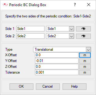
Define.
In the Periodics BC dialog, select the surfaces Side1 and
Side2, respectively.
Verify that Type is Translational.
Set the Y-Offset to -0.01 m (which is the distance
between Side1 and Side2).
Figure 18.
Transformation information should be provided so that the Side 1 surface
after transformation matches the Side 2 surface. For the present case, Side 1
should be translated along (-Y) axis for a distance of 0.01m. Hence the Type as
Translational and the Y-Offset as -0.01m.
Click OK.
Check Periodic Boundary Conditions
The following steps define the periodic boundary conditions for various variables for
Side1 and Side2.
Click BAS in the Data Tree Manager to switch to basic view in the Data Tree.
Under Model, expand Periodics and expand
Side1-Side2.
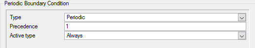
Make sure that the Periodic Boundary Condition box is checked On.
Double-click Periodic Boundary Condition and verify that
Type is set to Periodic and Active Type is set to Always.
Figure 19.
Set Nodal Output Frequency
The Nodal Output Frequency determines at what frequency or time interval the solution
results would be stored to be used for post processing within AcuFieldView.
In the Data Tree, under Global, double-click
Output.
Double-click Nodal Output to open the detail panel.
Enter 2 as the Time step frequency.
This value indicates that AcuSolve should write results
every 2 time steps.
Turn Output initial condition on.
This indicates that AcuSolve writes initial conditions.
Save the database.
Compile the UDF
A UDF in the form of C language (wave.c) is provided with the tutorial. This C
program should be compiled using the following steps.
To compile the UDF on Windows:
Start AcuConsole Command
Prompt from the Windows Start menu by clicking Start > All Programs > Altair Hyperworks <version> > AcuSolve > AcuSolve Cmd Prompt.
Use the cd command to change the directory to the
current working directory.
Enter the command acuMakeDll –src wave.c.
To compile the UDF on Linux:
In the terminal, use the cd command to change the
directory to the current working directory.
Enter the command acuMakeLib -src wave.c.
A set of files necessary for
the use of UDF are created.
Assign Mesh Controls
Set Global Mesh Parameters
Now that the simulation characteristics have been set for the whole problem, the next
step is to generate the mesh.
Global mesh attributes are the meshing parameters applied to
the model as a whole without reference to a specific geometric volume, surface,
edge, or point. Local mesh attributes are used to create mesh generation controls
for specific geometry components of the model.
In the next steps you will set the global mesh attributes.
Click MSH in the Data Tree Manager to filter the
settings in the Data Tree to show only the controls
related to meshing.
Expand the GlobalData Tree item.
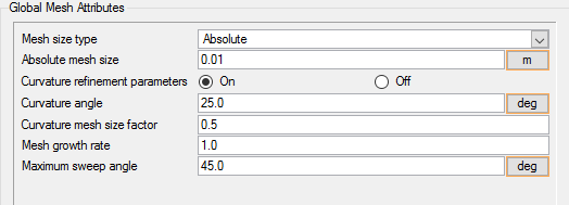
Double-click Global Mesh Attributes to open the
Global Mesh Attributes detail panel.
Change the Mesh size type to Absolute.
Enter 0.01 m for the Absolute mesh size.
Figure 20.
Define Mesh Extrusion
The present simulation is equivalent to a 2D representation of the model. In AcuSolve, 2D models are simulated by having just one element
across the thickness. In this case, there has to be only one element between Side1
and Side2. This can achieved with mesh extrusion process. Since you are using
identical boundary conditions on Side1 and Side2, using one element between them
will ensure that there is no variation in nodal values across thickness and hence
ensuring the simulation of a 2D model. In the following steps you will define the
process of extrusion of the mesh from Side1 to Side2.
Expand the ModelData Tree item and right-click Mesh
Extrusions.
Select New from the context menu to create a new entity,
Mesh Extrusion 1.
Rename Mesh Extrusion 1 as Side1-Side2.
Right-click Side1-Side2 and select
Define from the context menu.
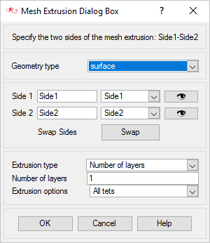
In the Mesh Extrusion dialog, make the following
settings.
Use the drop down arrows to select the surfaces for Side 1 and Side 2
as Side1 and Side2,
respectively.
Ensure that the Extrusion type is set to Number of layers.
Set Number of layers equal to 1.
Set Extrusion options to All tets.
Use the following figure for reference.
Click OK to close the dialog.
Generate the Mesh
In the next steps you will generate the mesh that will be used when computing a
solution for the problem.
Click on the toolbar to open the Launch
AcuMeshSim dialog.
For this case, the default settings will be used.
Click Ok to begin meshing.
During meshing an AcuTail window opens. Meshing
progress is reported in this window. A summary of the meshing process indicates that the
mesh has been generated.
Figure 21.
Note: The actual number of nodes and elements, and memory usage may vary
slightly from machine to machine.
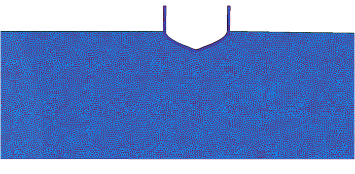
Visualize the mesh in the modeling window. Turn on the
display of surfaces, and set the display type to solid and
wire.
Figure 22.
Split Nodes
At this point, the Hull_guide surface has all nodes that are attached to Fluid. A
duplicate set of nodes has to be created, so that one set of the nodes follow the
Fluid motion and another set stays attached to the surface Guide_surf. The following
steps illustrate the process of splitting the nodes.
In the Data Tree, under Surfaces, right-click
Hull_guide and select Mesh Op. > Split internal faces.
There is an increase in the number of nodes.
Compute the Solution and Review the Results
Run AcuSolve
In the next steps you will launch AcuSolve to compute the solution for this case.
Click on the toolbar to open the
Launch AcuSolve dialog.
For this case, the default values will be used.
AcuSolve will run using four processors (if
available, higher number of processors may be specified) and AcuConsole will generate AcuSolve input files and will launch AcuSolve. AcuSolve will
calculate the transient solution for this problem.
Click Ok to start the
solution process.
While computing the solution, an
AcuTail window opens. Solution progress is
reported in this window. A summary of the solution process indicates
that the run has been completed.
The information provided in the summary is based on
the number of processors used by AcuSolve.
If you use a different number of processors than indicated in this
tutorial, the summary for your run may be slightly different than the
summary shown.
Figure 23.
Close the AcuTail window and save the database to create a
backup of your settings.
Monitor the Solution with AcuProbe
AcuProbe can be used to monitor various variables over
solution time. In the present simulation it is worthwhile to monitor the forces on
the ship hull.
Open AcuProbe by clicking on the toolbar.
In the Data Tree on the left, expand Surface Output > Hull_guide > Forces and Moments.
Right-click on x_wall_shear_stress and select
Plot.
Note: You might need to click on the toolbar in order to
properly display the plot.
Similarly, right-click on z_wall_shear_stress and click
on Plot.
Figure 24.
You can also save the plots as an image.
From the AcuProbe dialog, click File > Save.
Enter a name for the image and click
Save.
The time series data of the variables can also be exported as a text file
for further post-processing.
Right-click on the variable that you want to export and click
Export.
Enter a File name and choose .txt for
the Save as type.
Click Save.
View Results with AcuFieldView
Now that a solution has been calculated, you are ready to view
the flow field using AcuFieldView. AcuFieldView is a third-party post-processing tool
that is tightly integrated to AcuSolve. AcuFieldView can be started directly from AcuConsole, or it can be started from the Start menu, or from
a command line. In this tutorial you will start AcuFieldView from AcuConsole
after the solution is calculated by AcuSolve.
In the following steps you will start AcuFieldView and create an
animation of the ship hull motion with the contours of z-mesh displacement.
Start AcuFieldView
Click on the
AcuConsole toolbar to open the
Launch AcuFieldView dialog.
Click Ok to start
AcuFieldView.
When you start AcuFieldView from AcuConsole, the results from the last time step of the
solution that were written to disk will be loaded for post-processing.
View Water Displacement Around the Ship
These steps are provided with the assumption that you are able to manipulate the view
in AcuFieldView to have a white background, perspective
turned off, outlines turned off, and the viewing direction set to +z. If you are
unfamiliar with basic AcuFieldView operations, refer to
Manipulate the Model View in AcuFieldView.
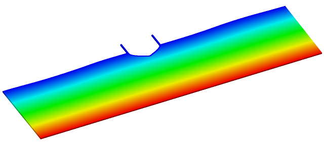
Orient the geometry so you can see the Top surface clearly, as shown in the
figure below.
Figure 25.
In the Boundary Surface dialog, uncheck Show Mesh.
Select z-mesh-displacement as the scalar function and
click Calculate.
In the Legend tab, click Show Legend.
Change the color to black.
Note: You can move the legend using Shift +
left-click.
From the Colormap tab, turn on Local.
Click Tools > Flipbook Build Mode and click OK .
Click Tools > Transient Data and move the slider all the way back to reflect the first time
step data on the boundary surfaces.
Click Build to build the animation.
Once the animation is built, click Frame Rate and change
it to 0.1.
Save the animation as Z-Displacement.
Summary
In this tutorial, you worked through a basic workflow to set up a static ship-hull simulation
with surface gravity waves. Once the case was set up, you generated a mesh and obtained a
solution using AcuSolve. Results were post-processed in AcuFieldView to allow you to create an animation of the free surface movement
with time. New features introduced in this tutorial include:
User Defined Function (UDF) for surface gravity wave generation
Mesh extrusions and periodic boundary conditions
ALE based mesh motion approach
Use of the Surface Manager to apply surface attributes
Use of hydrostatic pressure as a boundary condition
Free surface and Guide surface capabilities in AcuSolve


 on the toolbar.
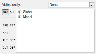
 on
the toolbar.
on
the toolbar.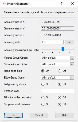

 .
.
 and
and  next to the volume name.
Note: You may not see any change when toggling the display if Surfaces are being displayed, as surfaces and volumes may overlap.
next to the volume name.
Note: You may not see any change when toggling the display if Surfaces are being displayed, as surfaces and volumes may overlap.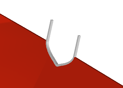

 on the toolbar to open the Launch
AcuMeshSim dialog.
For this case, the default settings will be used.
on the toolbar to open the Launch
AcuMeshSim dialog.
For this case, the default settings will be used.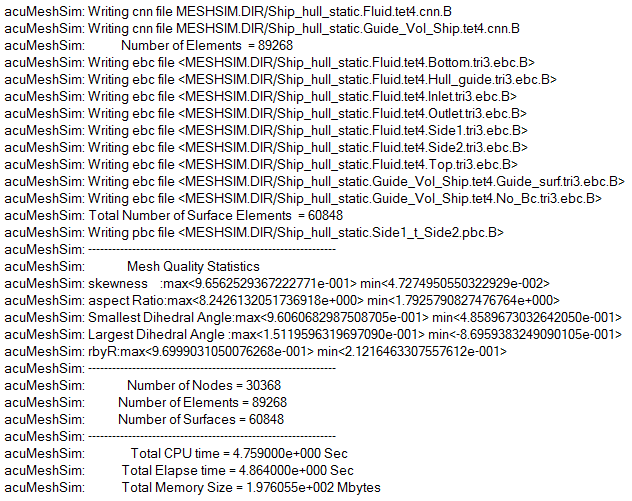
 on the toolbar to open the
Launch AcuSolve dialog.
For this case, the default values will be used.
on the toolbar to open the
Launch AcuSolve dialog.
For this case, the default values will be used.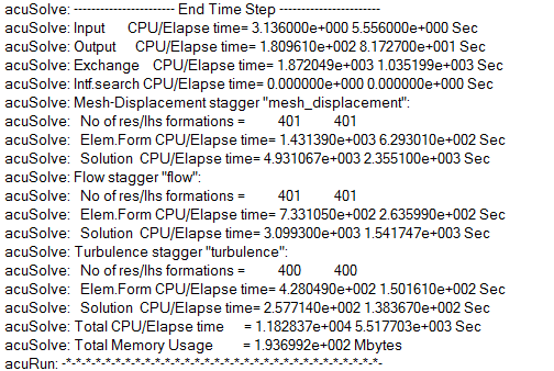
 on the toolbar.
 on the toolbar in order to
properly display the plot.
on the toolbar in order to
properly display the plot.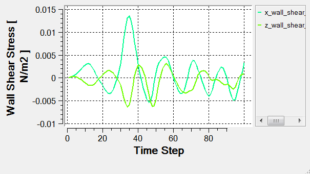
 on the
AcuConsole toolbar to open the
Launch AcuFieldView dialog.
on the
AcuConsole toolbar to open the
Launch AcuFieldView dialog.