ACU-T: 5202 Flow Closing Valve
This tutorial provides the instructions for setting up, solving and viewing results for a simulation of a flow closing valve. In this simulation, AcuSolve is used to set up the motion of the valve from open to a fully closed configuration. This tutorial is designed to introduce you to modelling concepts necessary to perform mesh motion simulations involving near contact simulations.
The basic steps in any CFD simulation are shown in the ACU-T: 2000 Turbulent Flow in a Mixing Elbow. The basic steps involving rigid body mesh motion are shown in the ACU-T: 5200 Rigid-Body Dynamics of a Check Valve. The following additional capabilities of AcuSolve are introduced in this tutorial:
- Creating a mesh motion with mesh distortion correction
- Creating advanced solution strategy parameters for mesh displacement stagger
- Creating multiplier function for translational mesh motion in terms of velocity or displacement
- Using the ogden model associated with Arbitrary Lagrangian Eulerian (ALE) mesh movement technology to run the simulation
In this tutorial, you will do the following:
- Analyze the problem
- Start AcuConsole and work with an existing database
- Set advanced simulation parameters
- Create a mesh motion to simulate near contact
- Assign mesh distortion correction parameters
- Create a multiplier function associated with velocity or, alternatively, displacement
- Edit the configuration file to run AcuSolve using the ogden ALE
- Monitor the solution with AcuProbe
- Post processing the time series output with AcuProbe
- Post processing the nodal output with AcuFieldView
Prerequisites
In order to run this tutorial, you should have already run through the introductory tutorial, ACU-T: 2000 Turbulent Flow in a Mixing Elbow and ACU-T: 5200 Rigid-Body Dynamics of a Check Valve tutorial. It is assumed that you have familiarity with AcuConsole, AcuSolve, and AcuFieldView. You will also need access to a licensed version of AcuSolve.
Prior to running through this tutorial, copy AcuConsole_tutorial_inputs.zip from <Altair_installation_directory>\hwcfdsolvers\acusolve\win64\model_files\tutorials\AcuSolve to a local directory. Extract Closing_Valve.acs from AcuConsole_tutorial_inputs.zip.
Analyze the Problem
An important step in any CFD simulation is to examine the engineering problem at hand and determine the important parameters that need to be provided to AcuSolve. Parameters can be based on geometrical elements (such as inlets, outlets, or walls) and on flow conditions (such as fluid properties, velocity, or whether the flow should be modeled as turbulent or as laminar).
The problem to be addressed in this tutorial is shown schematically in Figure 1. It consists of a rectangular channel with two flow paths, one of which may be closed by a valve.
The inlet height is 0.2 meters and the length of the domain is 1.0 meter. The initial position of the valve is at 9.165 millimeters from the opening, thus simulating an open condition.
The valve moves at a constant speed of 18.33 mm/s towards and away from the opening during a time duration of 1 second.

Figure 1. Schematic of the channel with one closing valve
Note that AcuSolve cannot simulate near contact configuration with the default settings. The mesh distortion correction and mesh stagger parameters need to be tweaked to allow the mesh elements to collapse and recover given sufficient iterations.
Define the Simulation Parameters
Start AcuConsole and Open the Existing Simulation Database
In the next steps you will start AcuConsole and open the existing database for storage of additional simulation settings. In this tutorial, you will begin by opening a database, creating advanced simulation settings for flow, turbulence, and mesh stagger, and creating the required mesh motion. Next, you will create a multiplier function based on velocity or displacement, modify mesh distortion parameters, and assign the mesh motion to the moving surface. Then, you will run AcuSolve to solve for the number of time steps specified. Finally, you will visualize some characteristics of the results using AcuFieldView.
-
Click to bring up the Open data base dialog.
Note: You can also bring up the Open data base dialog by clicking
 on the toolbar.
 -
Select Closing_Valve.acs and click
Open to open the database.
Note: In order for other applications to be able to read the files written by AcuConsole, the database path and name should not include spaces.
Once you open the database, you will notice that the geometry, mesh, simulation settings, and most of the boundary conditions have already been populated in the file.
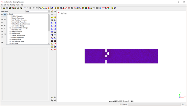
Figure 2.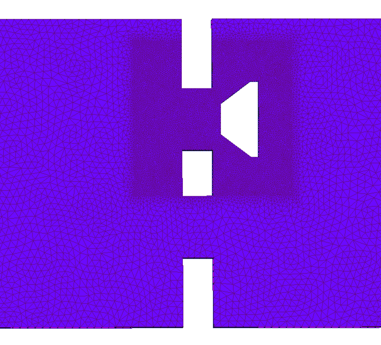
Figure 3.
Set Advanced Simulation Parameters
In the database, the general simulation, solution strategy, material model, and mesh parameters have already been created.
In next steps, you will create and set the advanced solution strategy parameters that apply to the simulation. To make this as simple as possible, you will use the PB* filter in the Data Tree Manager. This filter reduces the number of items shown in the Data Tree and makes navigation of the entries easier.
-
Under the Global Data Tree item, double-click
Advanced Solution Strategy, then double-click the
Stagger tree.
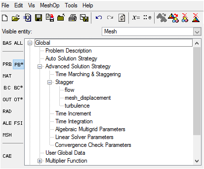
Figure 4.The advanced solution strategy tree contains settings that can be used to finely tune the solver parameters, such as time increment, time marching, staggers, linear solver, convergence check, etc.
The stagger command specifies the nonlinear iteration and linear solver parameters for the solution of an equation. Each stagger loops over several nonlinear iterations, within which the residual, and optionally, the LHS matrix of the stagger are formed, the resulting linear equation system is solved, the corresponding solution field is updated, and its sub-staggers are executed.
-
Set the Convergence tolerance to 0.01.
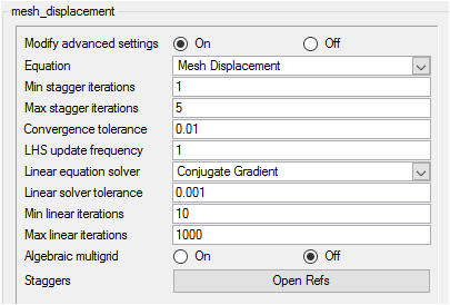
Figure 5.
Assign Mesh Controls
Create a Multiplier Function
- Click PB* in the Data Tree Manager to display all the available settings related to general problem setup in the Data Tree.
- Expand the Global Data Tree item.
- Create a new multiplier function named Velocity_Multiplier.
-
Define the multiplier function parameters.
-
Click the drop-down control next to Curve fit variable and select
Time step.
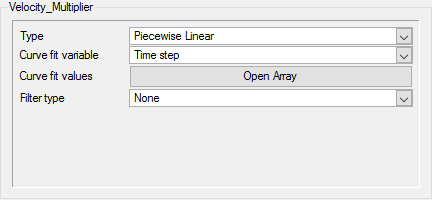
Figure 6. -
Click Plot << to see the plot of the
multiplier function.
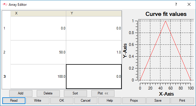
Figure 7.
-
Click the drop-down control next to Curve fit variable and select
Time step.
Create Velocity-Based Mesh Motion
AcuSolve uses the mesh motion command to define the movement of nodes within the model. In this tutorial, you will use a translational mesh motion to determine the motion of the nodes.
A multiplier function is used to scale values as a function of time or time step. In this tutorial, the stop valve moves towards and away from the opening at a constant speed. This variation is accomplished by assigning a multiplier function to the mesh motion.
In the next steps, you will create a mesh motion to simulate the motion of the valve.
- Click FSI in the Data Tree Manager to filter the settings in the Data Tree to show only those related to mesh motions and fluid/structure interactions.
- Double-click the Global Data Tree item to expand it.
- Right-click Mesh Motion and click New.
-
Rename the mesh motion.
- Right-click Mesh Motion 1.
- Click Rename.
- Type Valve_Motion and press Enter
-
Define the mesh motion parameters.
-
Change the units to mm/sec and enter
-18.33 in the X-component field.
This corresponds to the x component of the velocity defining the mesh motion.
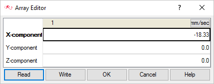
Figure 8. -
Click the drop-down next to Velocity variable and select
Multiplier function.
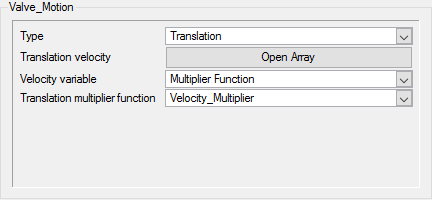
Figure 9.A new option called Translation multiplier function becomes available.
-
Change the units to mm/sec and enter
-18.33 in the X-component field.
When this translation mesh motion is defined, the nodes of the element set move at a constant velocity of 18.33 mm/s in the negative x direction. For this case, the location of each node in the element set is given by:
Where is the initial condition of the node, is given by translation velocity, and is time.
A multiplier function can be defined with velocity_variable=multiplier_function to modify the scaling of velocity. Then the location of each node is given by:
Where is the given translation variable multiplier function.
Create Displacement-Based Mesh Motion
An alternate approach for defining a multiplier function for translation mesh motion is to define a unit (1.0) velocity value in the mesh motion and assign the displacement of the moving body to the multiplier function directly.
This approach is particularly useful in cases where you are given the displacement-time values or curves defining the motion of the moving body.
In the next steps, you will define the mesh motion and multiplier function based on the approach discussed in previous sections.
-
Set the X-velocity to 1.0 m/sec in the X-component field
of the array editor.
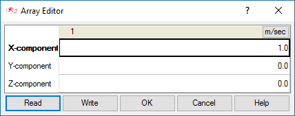
Figure 10. -
Enter the displacement values for the curve fit variables in the array editor,
as shown in the image below.
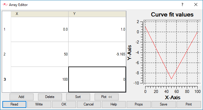
Figure 11.This approach allows you to define the motion of the valve based on the displacement against the time steps.
Assign Mesh Distortion Parameters
When AcuSolve is performing a moving mesh simulation, a check is performed to detect the presence of bad elements. If any highly distorted element are found, the code either exits (when mesh=specified or mesh=eulerian) or adds more non-linear iterations with an incremental update strategy (when mesh=ale). Two parameters control the algorithm: mesh_distortion_tolerance and mesh_distortion_correction_factor. The first parameter determines whether the correction needs to be applied to the element Jacobian and the second quantifies the amount of correction. Mesh distortion is checked within the ALE loop, and then acuSolve decides how forgiving it should be to highly distorted elements.
In the next steps you will assign the values of mesh distortion parameters to the fluid volume.
-
Enter 0.05 as the value for the Mesh distortion
tolerance.
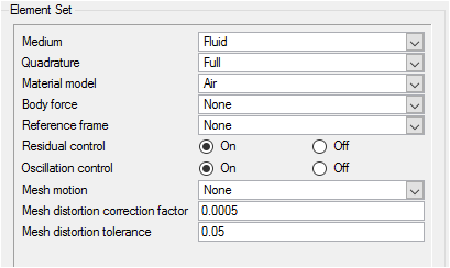
Figure 12.
Assign Mesh Motion to the Valve Surface
Surface groups are containers used for storing information about a surface, including solution and meshing parameters, and the corresponding surface in the geometry that the parameters will apply to.
The database has all the volume and surface groups already assigned.
In the next steps, you will assign the created mesh motion to the valve surface.
-
Click the drop-down menu next to Mesh motion and select
Valve_Motion.
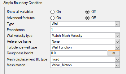
Figure 13.
Compute the Solution and Review the Results
Run AcuSolve
In order to use the ogden model associated with Arbitrary Lagrangian Eulerian (ALE) mesh movement technology, you need to add the corresponding flag in the configuration file and then run the simulation using the AcuSolve command prompt.
In the next steps, you will run AcuPrep from the GUI, edit the configuration file, and launch AcuSolve from the command prompt in order to get a solution for this case.
-
Click
 on the toolbar to open the
Launch AcuSolve dialog.
For this case, only the AcuPrep module will be used, and AcuConsole will generate AcuSolve input files and launch AcuSolve.
on the toolbar to open the
Launch AcuSolve dialog.
For this case, only the AcuPrep module will be used, and AcuConsole will generate AcuSolve input files and launch AcuSolve. -
From the drop-down menu next to Solver modules, select
prep.
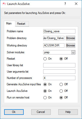
Figure 14. -
Launch AcuSolve with the command AcuRun -np 4 -nt 1
-do solve to run the simulation with four processors and only the
solver module.
Note: The solution progress can be monitored by launching AcuTail using the
 icon from the toolbar and selecting the log file from your working
directory.After AcuSolve has finished running, a summary of the solution process indicates that the simulation has been completed.
icon from the toolbar and selecting the log file from your working
directory.After AcuSolve has finished running, a summary of the solution process indicates that the simulation has been completed.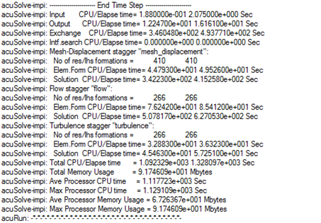
Figure 15.
Post Process with AcuProbe
After the simulation is complete, the plot for mesh_x_displacement can be viewed using AcuProbe.
-
Open AcuProbe by clicking
 on the toolbar.
-
Right-click on mesh_x_displacement and click
plot.
Note: You might need to click
 on the toolbar in order to
properly display the plot.
on the toolbar in order to
properly display the plot.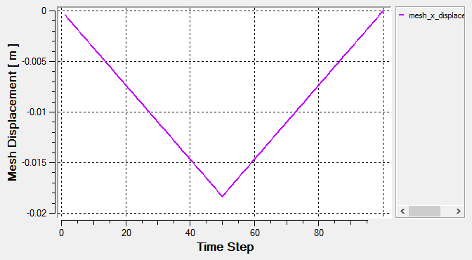
Figure 16.Other flow quantities can also be plotted using AcuProbe.
View Results with AcuFieldView
Now that a solution has been calculated, you are ready to view the flow field using AcuFieldView. AcuFieldView is a third-party post-processing tool that is tightly integrated to AcuSolve. AcuFieldView can be started directly from AcuConsole, or it can be started from the Start menu, or from a command line. In this tutorial you will start AcuFieldView from AcuConsole after the solution is calculated by AcuSolve.
In the following steps you will start AcuFieldView, display velocity magnitude and animate the view to show mesh displacement. You will then display velocity vectors and pressure contours when the valve shutter is closed.
- How to find the data readers in the File pull-down on the Main menu and open up the desired reader panel for data input.
- How to find the visualization panels either from the Side toolbar or the Visualization panel pull-downs on the Main menu to create and modify surfaces in AcuFieldView.
- How to move the data around the graphics window using mouse actions to translate, rotate and zoom in to the data.
This tutorial shows you how to work with transient data. It also shows how to visualize the flow parameters on the complete geometry when only a section of it is simulated in AcuSolve by using multiple datasets.
Start AcuFieldView
-
Click
 on the
AcuConsole toolbar to open the
Launch AcuFieldView dialog.
on the
AcuConsole toolbar to open the
Launch AcuFieldView dialog.
-
Click Ok to start
AcuFieldView.
When you start AcuFieldView from AcuConsole, the results from the last time step of the solution that were written to disk will be loaded for post-processing.
Once AcuFieldView opens, you will see that the pressure contours have already been displayed on all the boundary surfaces with mesh.
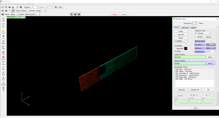
Figure 17.
Animate the Display of Velocity Magnitude Contours
In the next steps you will create a transient sweep and save it as an animation that can be viewed independently of AcuFieldView.
-
Turn off the display for the mesh by unchecking the Show Mesh option under the
Surfaces tab.
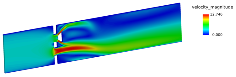
Figure 18. -
Go to and move the slider all the way back to reflect the first time
step data on the boundary surface.
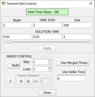
Figure 19.
Display Pressure Contours and Velocity Vectors on a Mid-Z Coordinate Surface at Valved Closed Position
-
Change the view to +Z from the Defined Views menu.
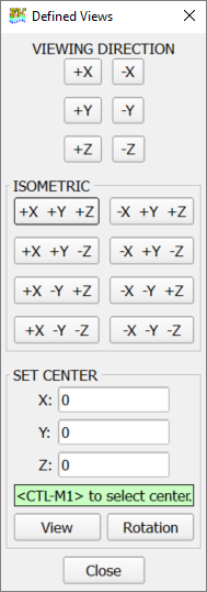
Figure 20. -
Click
 to open
the Coordinate Surface dialog.
to open
the Coordinate Surface dialog.
-
Set Scalar Coloring to Local from the Colormap
tab.
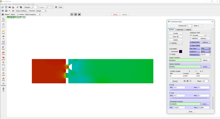
Figure 21. -
Check Skip and enter 62.5%.
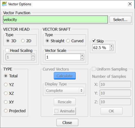
Figure 22. -
Go to and move the slider to the 50th time step.
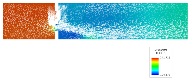
Figure 23.