ACU-T: 5201 Coupled Simulation of a Check Valve using AcuSolve and MotionSolve
Prerequisites
This tutorial introduces you to the workflow for setting up an AcuSolve-MotionSolve co-simulation using HyperMesh Desktop. Prior to starting this tutorial, you should have already run through the introductory HyperWorks tutorial, ACU-T: 1000 HyperWorks UI Introduction, and have a basic understanding of HyperMesh, AcuSolve, and HyperView. To run this simulation, you will need access to a licensed version of HyperMesh and AcuSolve.
Prior to running through this tutorial, copy HyperMesh_tutorial_inputs.zip from <Altair_installation_directory>\hwcfdsolvers\acusolve\win64\model_files\tutorials\AcuSolve to a local directory. Extract ACU-T5201_CheckValveCoupled.hm and Valve_model.xml from HyperMesh_tutorial_inputs.zip.
Since the HyperMesh database (.hm file) contains meshed geometry, this tutorial does not include steps related to geometry import and mesh generation.
Problem Description

Figure 1. Schematic of Check Valve with Spring-Loaded Shutter
The pipe has an inlet diameter of 0.08 m and is 0.4 m long. The check-valve assembly is 0.085 m downstream of the inlet. It consists of a plate 0.005 m thick with a centered orifice 0.044 m in diameter and a shutter with an initial position 0.005 m from the opening, simulating a nearly closed condition. The shutter plate is 0.05 m in diameter and 0.005 m thick. The shutter plate is attached to a stem 0.03 m long and 0.01 m in diameter. The mass of the shutter and stem is 0.2 kg and its motion is affected by a virtual spring with a stiffness of 2162 N/m. The motion of the valve shutter is limited by a stop mounted on a perforated plate downstream of the shutter.
Modeling the geometry as a 30° section requires that the fluid model is set up to be consistent with the rigid-body model. Since only 1/12 of the rigid body is modeled, the forces computed by AcuSolve that act on the valve shutter represent 1/12 of the actual force on the device. The rigid-body-dynamics model was set up in MotionSolve with scaled settings of mass and spring stiffness to account for the fact that you are only modeling a small section of the full geometry. Additional information regarding the setup of this problem in MotionSolve is provided in the MotionSolve documentation.
The fluid in this problem is water, which has a density (ρ) of 1000 kg/m3 and a molecular viscosity (μ) of 1 X 10⁻³.
At the start of the simulation the flow field is stationary. Flow is driven by the pressure at the inlet, which varies over time as a piecewise linear function shown in Figure 2. As the pressure at the inlet rises, the flow will accelerate as the valve opens. The turbulence viscosity ratio is assumed to be 10.
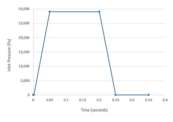
Figure 2. Transient pressure at the inlet
Prior simulations of this geometry indicate that the average velocity at the inlet reaches a maximum of 0.98 m/s. At this velocity, the Reynolds number for the flow is 78,400. When the Reynolds number is above 4,000 it is generally accepted that flow should be modeled as turbulent. Mesh motion will be modeled using arbitrary mesh movement (arbitrary Lagrangian-Eulerian mesh motion).
For this case, the transient behavior of interest occurs in the time it takes for the pressure to ramp up and ramp back down, which is given by the transient pressure profile. To allow time for the spring to recover additional time will be simulated. For this tutorial 0.1 s is added after the pressure drops back to initial conditions for a total duration of 0.35 s.
Another critical decision in a transient simulation is choosing the time increment. The time increment is the change in time during a given time step of the simulation. It is important to choose a time increment that is short enough to capture the changes in flow properties of interest, but does not require unnecessary computation time. The change in inlet pressure from initial conditions to maximum occurs over 0.048 s. A time increment of 0.002 s would allow for excellent resolution of the transient changes without requiring excessive computational time.
Open the HyperMesh Model Database
-
Click the Open Model icon
 located on the standard
toolbar.
The Open Model dialog opens.
located on the standard
toolbar.
The Open Model dialog opens.
Set the General Simulation Parameters
Set the Analysis Parameters
-
Turn External Code On.
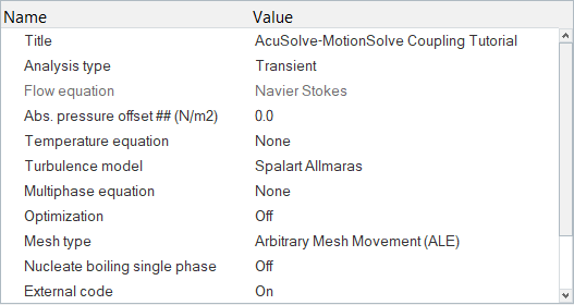
Figure 3.
Specify the Solver Settings
-
Turn External code On and verify that the Flow,
Turbulence and Mesh options are turned on.
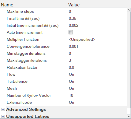
Figure 4.
Set External Code Parameters for Communication with MotionSolve
-
Enter 48000 as the Socket port.
This is the default port used for communication between AcuSolve and MotionSolve.
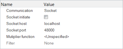
Figure 5.
Define the Nodal Output Frequency
-
In the Entity Editor, set the Time step frequency to
1.
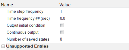
Figure 6.
Set the Boundary Conditions
Create a Multiplier Function for Inlet Pressure
-
In the Curve editor dialog, enter the following X,Y
values.
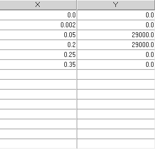
Figure 7. -
Verify that the Curve fit variable is set to Time and
the Evaluation Type is set to Per Time Step.
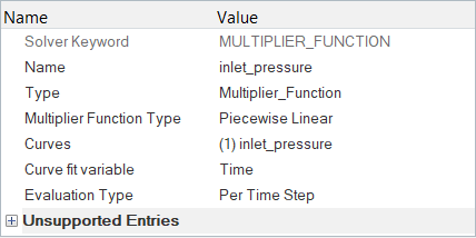
Figure 8.
Set the Boundary Conditions
-
Click Fluid. In the Entity Editor,
- Change the Type to FLUID.
- Set the Material to Water_HM.
- Leave the remaining default options.
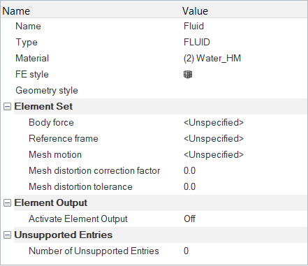
Figure 9. -
Click Inflow. In the Entity Editor,
- Change the Type to INFLOW.
- Turn On Show advanced features.
- Change the Inflow type to Stagnation Pressure.
- Set the Stagnation Pressure to 1 N/m2.
- Set the Stagnation Pressure multiplier function to inlet_pressure.
- Set the Turbulence input type to Viscosity Ratio.
- Set the Material to Water_HM in the top portion of the Entity Editor.
- Set the Turbulence viscosity ratio to 10.
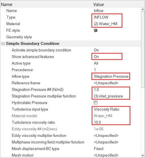
Figure 10. -
Click Outflow. In the Entity Editor, change the Type to
OUTFLOW.
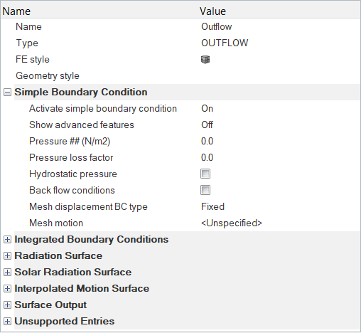
Figure 11. -
Click Valve_wall. In the Entity Editor,
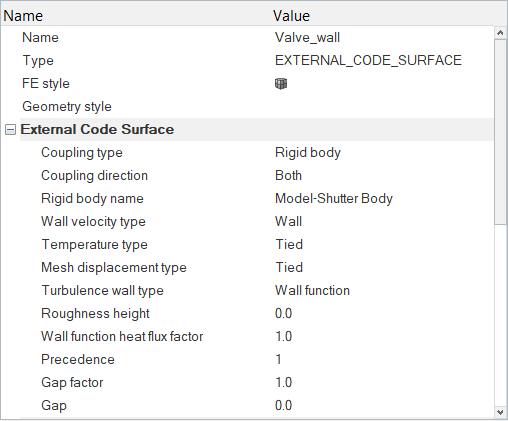
Figure 12. -
Click Outflow. In the Entity Editor, verify that the Type is set to
WALL.
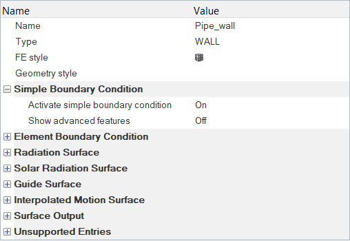
Figure 13. -
Click Front_symmetry. In the Entity Editor,
- Change the Type to SYMMETRY.
- Change the Mesh displacement BC type to Slip.
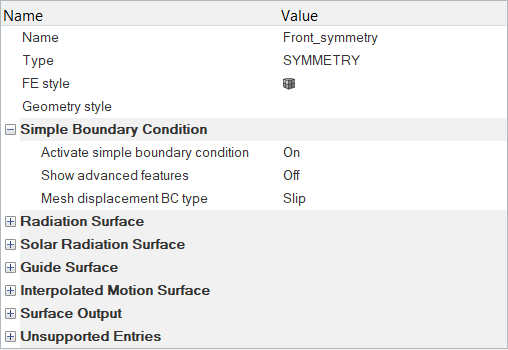
Figure 14.
Compute the Solution
- Start AcuSolve
- Start MotionSolve
The next sets of steps provide instructions for these two tasks.
Run AcuSolve
In this step, you will launch AcuSolve to compute a solution for this case.
-
Click
 on the ACU toolbar.
The Solver job Launcher dialog opens.
on the ACU toolbar.
The Solver job Launcher dialog opens. -
Leave the remaining options as
default and click Launch to start the solution
process.
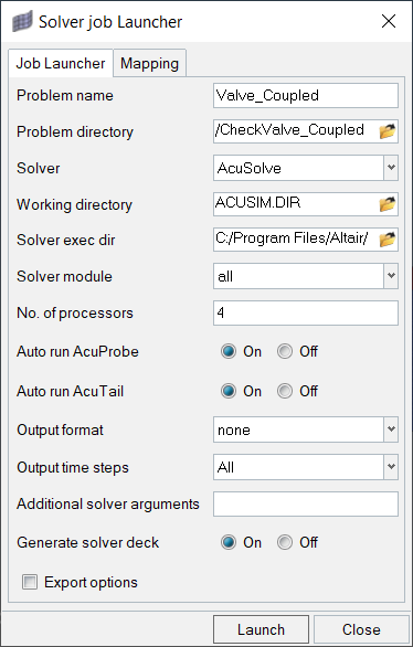
Figure 15.
Run MotionSolve
-
Click
 beside the Input file(s) field, browse to the location where you saved
Valve_model.xml, and open it.
beside the Input file(s) field, browse to the location where you saved
Valve_model.xml, and open it.
-
Click
 to
open the Available Options dialog.
to
open the Available Options dialog.
-
Enable the -as_cosim option to indicate coupling between
MotionSolve and AcuSolve.
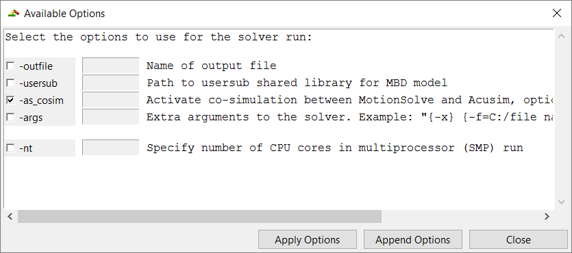
Figure 16. -
Click Run to start MotionSolve.
As the solution progresses, a HyperWorks Solver View window will open. Solution progress is reported in this window. The AcuSolve AcuTail window will also update as the solution progresses.
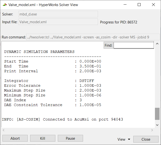
Figure 17.
Monitor the Solution with AcuProbe
Once the MotionSolve run launched, the AcuProbe window will be launched automatically after the first time step.
-
Right-click on mesh_x_displacement and select
Plot.
Note: You might need to click
 on the toolbar in order to
properly display the plot.
on the toolbar in order to
properly display the plot.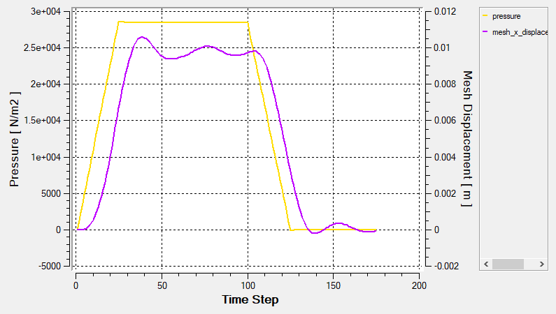
Figure 18.In the next steps you will create a plot of the x-velocity of the valve walls.
-
Expand , right-click on x_velocity, and select
Plot.
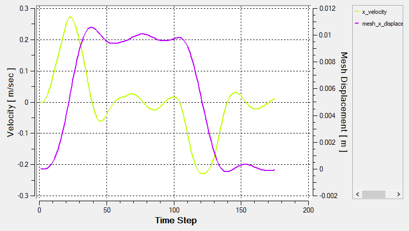
Figure 19.
Post-Process the Results with HyperView
In this step, you will create an animation of the valve motion as the water flows across the valve. Once the solver run is complete, close the AcuProbe and AcuTail windows. In the HyperMesh Desktop window, close the AcuSolve Control tab and save the model.
Switch to the HyperView Interface and Load the AcuSolve Model and Results
-
In the HyperMesh Desktop window, click the
ClientSelector drop-down in the bottom-left corner of
the graphics window.
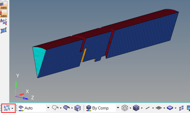
Figure 20. -
In the Load model and results panel, click
 next
to Load model.
next
to Load model.
Create an Animation of Velocity Magnitude
-
In the Results Browser, expand the list of
Components then click the Isolate
Shown icon
 .
.
-
Click the Front_symmetry component to turn off the
visibility of all the components except the front symmetry surface.
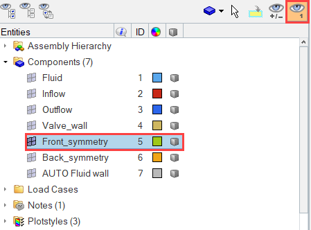
Figure 21. -
Orient the display to the xy-plane by clicking
 on the Standard Views toolbar.
-
Click
 on the Results toolbar to open the Contour panel.
-
In the panel area, under the Display tab, turn off
the Discrete color option.
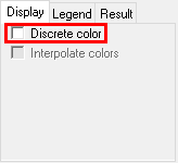
Figure 22. -
In the Edit Legend dialog, change the Type to
Dynamic scale and the Numeric format to
Fixed then click OK.
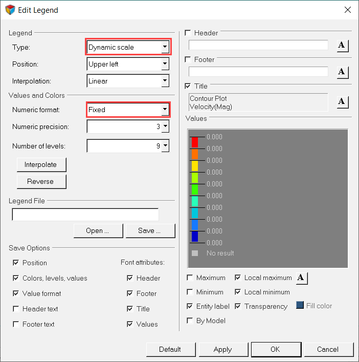
Figure 23. -
Click
 on the Animation toolbar to play the velocity magnitude
animation on the front symmetry plane.
on the Animation toolbar to play the velocity magnitude
animation on the front symmetry plane.
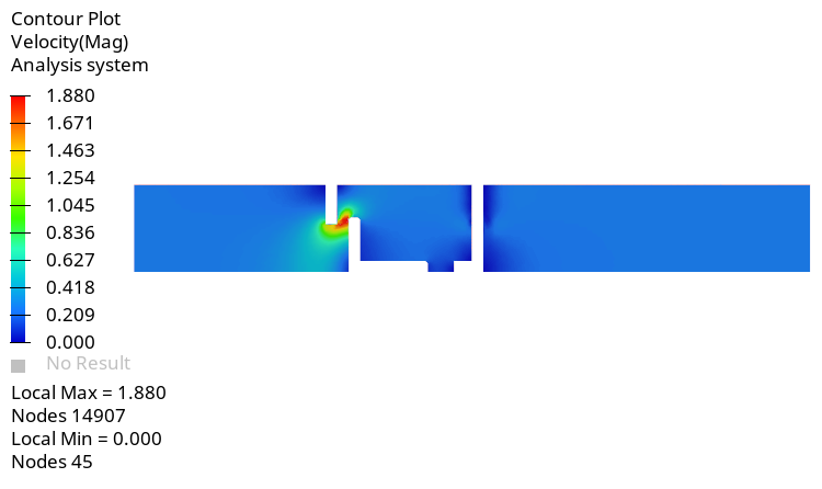
Figure 24. -
On the ImageCapture toolbar, click on the Capture Graphics Area
Video icon
 .
.
Display Pressure and Velocity Contours on a Section Cut
-
In the Results Browser, turn off the display of all the
Components except the Fluid component.
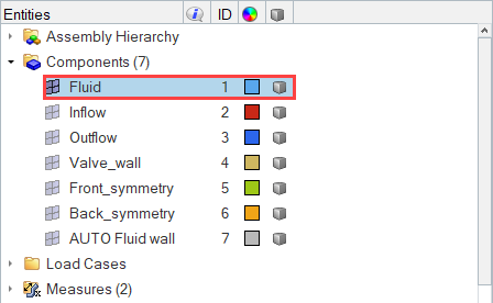
Figure 25. -
Click
on the Results toolbar to open the Contour panel.
-
In the panel area, under the
Result tab, activate the Overlay result
display check box (if not already selected).
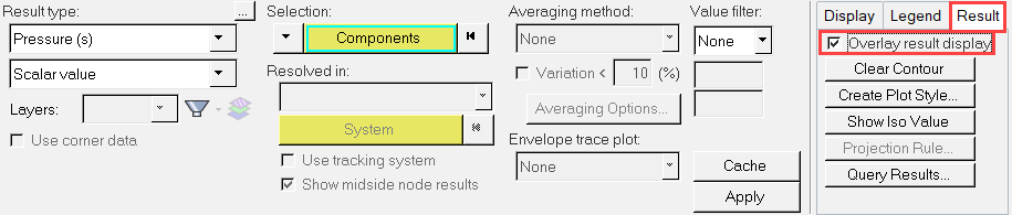
Figure 26. -
Click the Section cut icon
 on the HV-Display toolbar.
-
Click Gridline. In the Gridline
Options dialog, deactivate the Show check
box under Grid line then click OK.
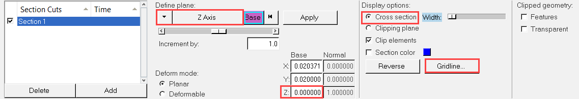
Figure 27. -
Click
 on the Results toolbar to open the Vector panel.
-
Click the Selection drop-down and select
Sections from the list of options.
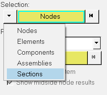
Figure 28. -
Set the Color by option to Direction and set the X+Y+Z
color to White.
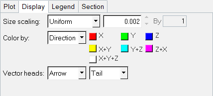
Figure 29. -
Go to the Section tab, activate the
Projected check box, then click
Apply.
The vector plot should look like the one shown in the figure below.
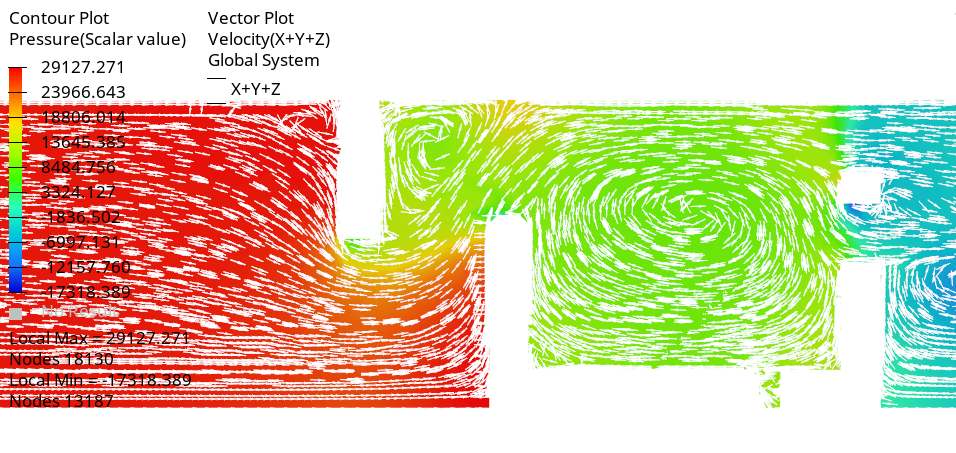
Figure 30.The result at 0.156 sec is shown.
Summary
In this tutorial, you learned the basic workflow to set up a co-simulation using AcuSolve and MotionSolve. The tutorial introduced you to the steps involved in setting up external code communication between AcuSolve and MotionSolve using HyperMesh Desktop and then running the simulation and post-processing the results using HyperView. You also learned how to create a vector plot on an existing contour plot on a cut plane.