ACU-T: 5100 Modeling of a Fan Component: Axial Fan
This tutorial provides the instructions for setting up, solving and viewing results for simulation of flow inside a pipe with an interior fan placed at the middle of the pipe. This middle portion of the pipe is considered to be fan volume which is modeled using the Fan_Component parameter. In this simulation, flow is passed from the pipe inlet and it enters the fan in axial direction and exits at the outlet causing pressure rise due to the fan. A lumped fan model is used to obtain fan pressure rise for a known inlet volume flow rate. This tutorial is designed to introduce the user to modeling concepts related to Fan_Components for axial fans.
- Specifying FAN_COMPONENT parameter in AcuConsole
- Setting up Inflow boundary condition with volumetric flow rate
Prerequisites
You should have already run through the introductory tutorial, ACU-T: 2000 Turbulent Flow in a Mixing Elbow. It is assumed that you have some familiarity with AcuConsole, AcuSolve, and AcuFieldView. You will also need access to a licensed version of AcuSolve.
Prior to running through this tutorial, copy AcuConsole_tutorial_inputs.zip from <Altair_installation_directory>\hwcfdsolvers\acusolve\win64\model_files\tutorials\AcuSolve to a local directory. Extract AxialFan.x_t from AcuConsole_tutorial_inputs.zip.
The color of objects shown in the modeling window in this tutorial and those displayed on your screen may differ. The default color scheme in AcuConsole is "random," in which colors are randomly assigned to groups as they are created. In addition, this tutorial was developed on Windows. If you are running this tutorial on a different operating system, you may notice a slight difference between the images displayed on your screen and the images shown in the tutorial.
Analyze the Problem

Figure 1. Axial Fan Model Used for the Simulation
Figure 1 shows a simple axial fan component problem where fan is an interior fan with thickness “t” and tip radius as “r”. In this simulation, flow is passed from the pipe inlet and it enters the fan in axial direction and exits at the outlet causing pressure rise due to the fan. This fan pressure rise can be simulated for a given volume flow rate at the inlet surface which will be assigned as the inflow boundary condition. The volume flow rate at the inlet surface is considered to be 525.35 m3/hr.
The middle portion of the pipe is the Fan Component volume which has both Fan_Inlet and Fan_Outlet. The FAN_COMPONENT parameters are assigned to Fan_Inlet surface through Advance problem definition option. Basically, the fan model is applied to a surface, and the pressure jumps across that surface to model the effect of the fan. The outlet of the pipe geometry is assigned with Outflow BC to model the flow exit whereas the outer walls are defined to be Wall BC with slip condition. The fluid material considered for this simulation is air with density=1.225 kg/m3, viscosity=1.781e-005 kg/m-s.
- Evaluate the flow rate at the inlet to the domain that is assigned as a fan component (that is, the surface on which you have assigned the FAN_COMPONENT condition)
- Evaluate the pressure rise resulting from this flow rate based on the fan curve that the user has input
- Compute a body force per unit length that yields the required pressure rise based on fan_length input parameter and the target pressure rise.
- The body force can be specified to be a function of the flow direction, that is, axial velocity, radial velocity, tangential velocity or combination of all these three.
- Assign the body force to all elements of the element set that the FAN_COMPONENT is assigned to.
So, when deciding how to set up the FAN_COMPONENT model, you also need to consider how your fan is modeled. If it is purely axial flow, then the relevant pressure rise relationship is just in the axial direction, and the fan_length is the distance from inlet to outlet of the fan section.
Basically the FAN_COMPONENT is modelled by adding axial, radial and tangential body forces to the momentum equations. For an axial fan type, these forces increase the pressure across the component by
where : axial coefficient
: density
: tip velocity =
: fan angular rotational speed (rad/sec)
: fan tip radius
: mass averaged velocity through the inlet (m/sec)
Since piecewise_bilinear curve fit values used in FAN_COMPONENT are functions of the normalized flow rate (Q1) and axial coefficient (αaxial), you need to convert them from the fan performance curve.
Normalized flow rate (Q1):
Axial co-efficient (αaxial) =
| Fluid Density | 1.225 kg/m3 |
| Tip Radius () | 0.11 m |
| Rotational Speed () | 3600 RPM = 376.99 rad/sec |
| Inlet Area, Ai | 0.03801 m2 |
| Tip Velocity () | 41.47 m/sec |
| Volume Flow Rate (Q), m3/hr | Pressure rise (ΔP), Pa | |
|---|---|---|
| 1 | 525.35 | 494.91 |
| 2 | 890.21 | 474.63 |
| 3 | 1161.63 | 424.9 |
| 4 | 1272.76 | 389.11 |
| 5 | 1356.57 | 350.42 |
| 6 | 1431.84 | 308.18 |
| 7 | 1494.69 | 268.35 |
| 8 | 1551.39 | 230.89 |
- For Q = 525.35 m3/hr:
Q1 = = 0.0926
= = 0.4613
- For Q = 890.21 m3/hr:
Q1 = = 0.1569
= = 0.426
| S. No | Normalized Flow Rate (Q1) | Axial Coefficients ( αaxial ) |
|---|---|---|
| 1 | 0.0926 | 0.4613 |
| 2 | 0.1569 | 0.426 |
| 3 | 0.2047 | 0.3615 |
| 4 | 0.2243 | 0.3191 |
| 5 | 0.2391 | 0.2755 |
| 6 | 0.2523 | 0.2289 |
| 7 | 0.2634 | 0.1854 |
| 8 | 0.2734 | 0.1445 |
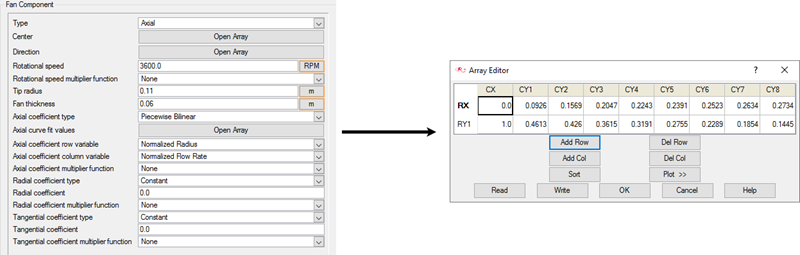
Figure 2. Fan Component Array Editor
The first column of array is the normalized radius which varies between 0 and 1 which implies that at the centre of the fan, this value is 0 whereas at the tip of the fan, this value is 1.
Define the Simulation Parameters
Start AcuConsole and Create the Simulation Database
In this tutorial, you will begin by creating a database, populating the geometry-independent settings, loading the geometry, creating volume and surface groups, setting group parameters, adding geometry components to groups, and assigning mesh controls and boundary conditions to the groups. Next you will generate a mesh and run AcuSolve to solve for the number of time steps specified. Finally, you will visualize some characteristics of the results using AcuFieldView.
In the next steps you will start AcuConsole, and create the database for storage of the simulation settings.
Set General Simulation Parameters
In next steps you will set parameters that apply globally to the simulation. To make this simple, the basic settings applicable for any simulation can be filtered using the BAS filter in the Data Tree Manager. This filter enables display of only a small subset of the available items in the Data Tree and makes navigation of the entries easier.
The physical models that you define for this tutorial correspond to steady state, turbulent flow.
-
Click BAS in the Data Tree Manager to switch to basic view in the Data Tree.
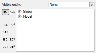
Figure 3. -
Double-click the Global
Data Tree item to expand it.
Tip: You can also expand a tree item by clicking
 next to the item name.
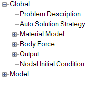
Figure 4. -
Change the Turbulence equation to Spalart
Allmaras.
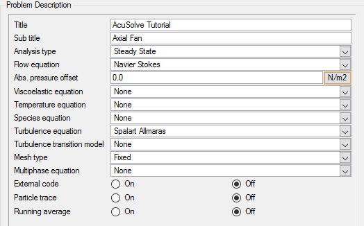
Figure 5.
Set Solution Strategy Parameters
In the next steps you will set parameters that control the behavior of AcuSolve as it progresses during the solution.
-
Check the Flow and Turbulence are set to On.
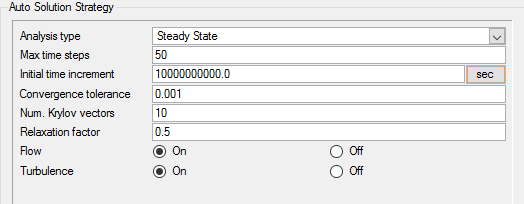
Figure 6. Auto Solution Detail Panel
Set Material Model Parameters
-
Double-click Material Model
in the Data Tree to expand it.
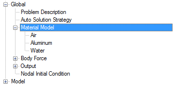
Figure 7. -
Save the database to create a backup
of your settings. This can be achieved with any of the following
methods.
- Click the File menu, then click Save.
- Click
 on
the toolbar.
on
the toolbar. - Click Ctrl+S.
Note: Changes made in AcuConsole are saved into the database file (.acs) as they are made. A save operation copies the database to a backup file, which can be used to reload the database from that saved state in the event that you do not want to commit future changes.
Import the Geometry and Define the Model
Import the Geometry
-
Select AxialFan.x_t and click
Open to open the Import Geometry
dialog.
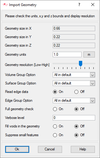
Figure 8.For this tutorial, the default values for the Import Geometry dialog are used to load the geometry. If you have previously used AcuConsole, be sure that any settings that you might have altered are manually changed to match the default values shown in the figure. With the default settings, volumes from the CAD model are added to a default volume group. Surfaces from the CAD model are added to a default surface group. You will work with groups later in this tutorial to create new groups, set flow parameters, add geometric components, and set meshing parameters.
-
Click Ok to complete
the geometry import.
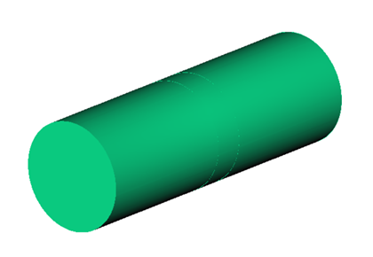
Figure 9.
Apply Volume Parameters
Volume groups are containers used for storing information about a volume region. This information includes the list of geometric volumes associated with the container, as well as attributes such as material models and mesh size information.
When the geometry was imported into AcuConsole, all volumes were placed into the "default" volume container.
In the next steps you will rename the default volume group container, assign the materials for that group, and set mesh motion for the fluid volume.
-
Expand Volumes. Toggle the display of the default
volume container by clicking
 and
and  next to the volume name.
Note: You may not see any change when toggling the display if Surfaces are being displayed, as surfaces and volumes may overlap.
next to the volume name.
Note: You may not see any change when toggling the display if Surfaces are being displayed, as surfaces and volumes may overlap. -
Rename Volume 1 and Volume 2, and set the columns as per the image below:
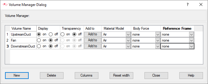
Figure 10. -
Assign the respective volumes to their volume groups:
-
Select the volume as shown in figure below and click
Done.
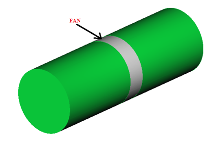
Figure 11. -
Select the volume as shown in figure below and click
Done.
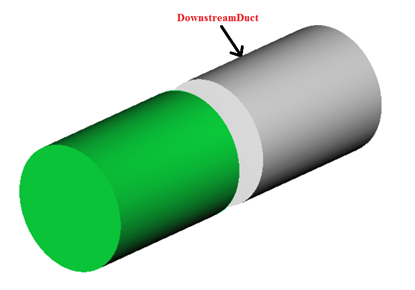
Figure 12.When the geometry was loaded into AcuConsole, complete geometry volume was placed in the default volume group. This default volume group was renamed to UpstreamDuct. In the previous steps, you assigned some volumes to various other volume groups that you created. At this point, all that is left is the UpstreamDuct volume group wherein the flow enters through the volume.
-
Repeat the process with UpstreamDuct.
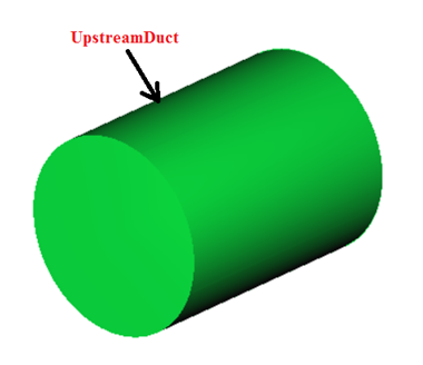
Figure 13.
-
Select the volume as shown in figure below and click
Done.
Create Surface Groups and Apply Surface Parameters
Surface groups are containers used for storing information about a surface, including solution and meshing parameters, and the corresponding surface in the geometry that the parameters will apply to.
In the next steps you will define surface groups, assign the appropriate settings for the different characteristics of the problem, and add surfaces to the group containers.
In the process of setting up a simulation, you need to move into different panels for setting up the boundary conditions, mesh parameters, and so on, which can sometimes be cumbersome, especially for models with too many surfaces. To make it easier, less error prone, and to save time, two new dialogs are provided in AcuConsole. Use the Volume Manager and Surface Manager to verify and provide the information for all surface or volume entities at once. In this section some features of Surface Manager are exploited.
-
If you cannot see the Simple BC Active and Simple BC Type columns, click on
Columns and select these two columns from the list and click Ok.
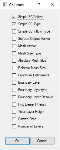
Figure 14. -
Set the Simple BC Active and Simple BC Type columns as per Figure 15.
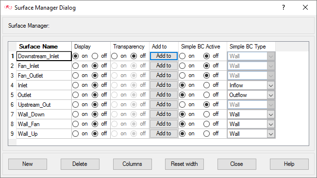
Figure 15. -
Assign the surfaces to the respective surface groups.
-
Select the planar symmetry surfaces as shown in the image, and click
Done.
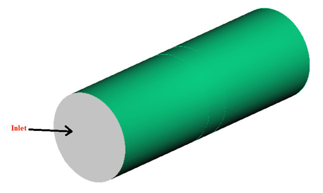
Figure 16. -
In the Outlet row, click Add to, and select the
surface shown below:
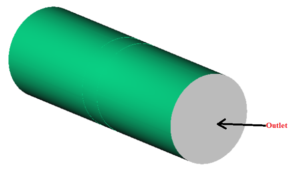
Figure 17. -
Assign the surface for the Wall_Up group.
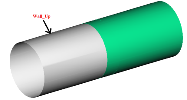
Figure 18. -
Assign the surface for the Wall_Fan group.
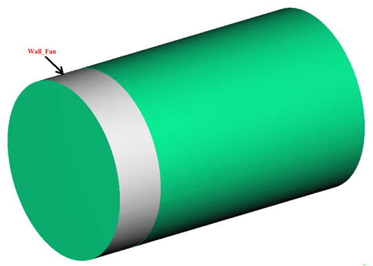
Figure 19. -
Assign the surface for the Wall_Down group.
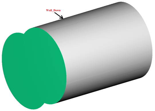
Figure 20. -
Assign the surface for the Upstream_Out group.
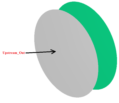
Figure 21. -
Assign the surface for the Fan_Inlet group.
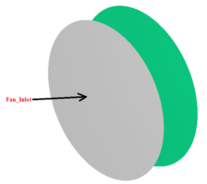
Figure 22. -
Assign the surface for the Fan_Outlet group.
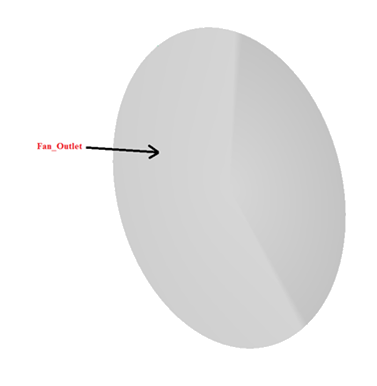
Figure 23.When the geometry was loaded into AcuConsole, all geometry surfaces were placed in the default surface group container. This default surface group was renamed to Downstream_Inlet. In the previous steps, you assigned some surfaces to various other surface groups that you created. At this point, all that is left is the Downstream_Inlet surface group which makes up the inlet of the DownstreamDuct volume.
-
Select the planar symmetry surfaces as shown in the image, and click
Done.
-
Assign the surface for the Downstream_Inlet group.
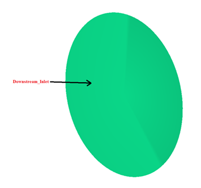
Figure 24.
Inlet
The Inlet group defines that the flow enters through the pipe and flows across length of the pipe. The correct boundary condition type for this surface is Inflow.
-
Enter the Flow rate value as 525.35.
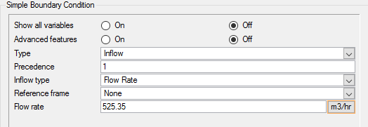
Figure 25.
Outlet
The Outlet group defines the exit of the pipe. The correct boundary condition type for this surface is Outflow.
-
Leave the remaining settings at their default values.
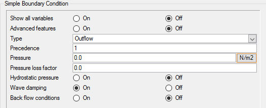
Figure 26.
Wall_Up
The walls enclose the fluid volume on the outside. The correct boundary condition type for this surface is Wall.
-
Leave the remaining settings at their default values.
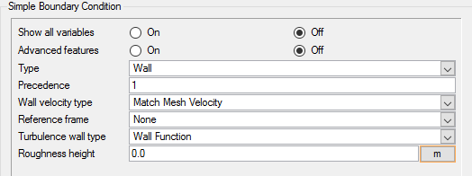
Figure 27.
Wall_Fan and Wall_Down
The surface groups Wall_Fan and Wall_Down will have the same settings as Wall_Up group. In order to not to repeat the steps again, you can propagate the settings to those two groups.
-
Click Propagate.

Figure 28.
Fan_Outlet
Upstream_Out
Downstream_Inlet
Fan_Inlet
-
Click Add Col seven times and enter the following as
shown in the figure below.
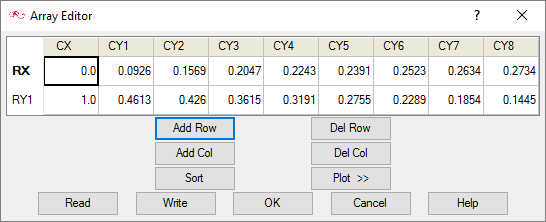
Figure 29. -
Leave the remaining settings at their default values.
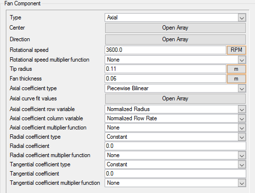
Figure 30.
Assign Mesh Controls
Set Global Mesh Parameters
Now that the flow characteristics have been set for the whole problem, a sufficiently refined mesh has to be generated.
Global mesh attributes are the meshing parameters applied to the model as a whole without reference to a specific geometric volume, surface, edge, or point. Local mesh attributes are used to create mesh generation controls for specific geometry components of the model.
In the next steps you will set the global mesh attributes.
-
Enter 0.0096 m for the Absolute mesh size.
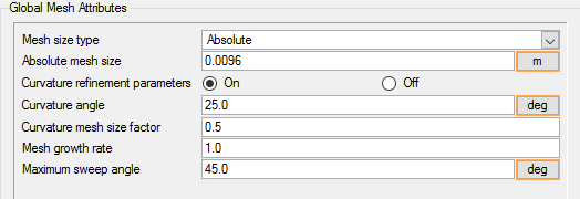
Figure 31.
Set Surface Mesh Parameters
Surface mesh attributes are applied to a specific surface in the model. It is a type of local meshing parameter used to create targeted mesh controls for one or more specific surfaces.
Setting local mesh attributes, such as surface mesh attributes, is not mandatory. When a local mesh attribute is not found for a component, the global attributes are used as the mesh generation control for that component. If a local mesh attribute is present, it will take precedence over the global setting.
In the next steps you will set the surface meshing attributes.
-
Leave the remaining settings at their default values.
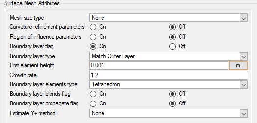
Figure 32.
The surface groups Wall_Fan and Wall_Down will have the same settings as the Wall_Up group. In order to not to repeat the steps again, you will propagate the settings to those two groups.
-
In the Propagate dialog, select the surface
Wall_Fan and Wall_Down, and
click Propagate.
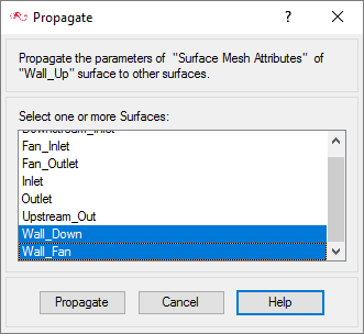
Figure 33.
Generate the Mesh
In the next steps you will generate the mesh that will be used when computing a solution for the problem.
-
Click
 on the toolbar to open the Launch
AcuMeshSim dialog.
For this case, the default settings will be used.
on the toolbar to open the Launch
AcuMeshSim dialog.
For this case, the default settings will be used. -
Click Ok to begin meshing.
During meshing an AcuTail window opens. Meshing progress is reported in this window. A summary of the meshing process indicates that the mesh has been generated.
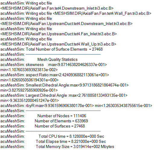
Figure 34.Note: The actual number of nodes and elements, and memory usage may vary slightly from machine to machine.
Compute the Solution and Review the Results
Run AcuSolve
In the next steps you will launch AcuSolve to compute the solution for this case.
-
Click
 on the toolbar to open the
Launch AcuSolve dialog.
For this case, the default settings will be used. AcuSolve will run using four processors (if available, higher number of processors may be specified) and AcuConsole will generate AcuSolve input files and will launch AcuSolve. AcuSolve will calculate the steady state solution for this problem.
on the toolbar to open the
Launch AcuSolve dialog.
For this case, the default settings will be used. AcuSolve will run using four processors (if available, higher number of processors may be specified) and AcuConsole will generate AcuSolve input files and will launch AcuSolve. AcuSolve will calculate the steady state solution for this problem. -
Click Ok to start the
solution process.
While computing the solution, an AcuTail window opens. Solution progress is reported in this window. A summary of the solution process indicates that the run has been completed.
The information provided in the summary is based on the number of processors used by AcuSolve. If you use a different number of processors than indicated in this tutorial, the summary for your run may be slightly different than the summary shown.
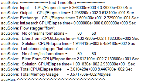
Figure 35.
Post-Process with AcuProbe
AcuProbe can be used to monitor various variables over solution time.
-
Open AcuProbe by clicking
 on the toolbar.
-
Right-click on Final and select Plot
All.
This will plot the residuals for the three variables - eddy viscosity, pressure and velocity in the plot area. This plot indicates the convergence of the variables with respect to timestep.Note: You might need to click
 on the toolbar in order to
properly display the plot.
on the toolbar in order to
properly display the plot.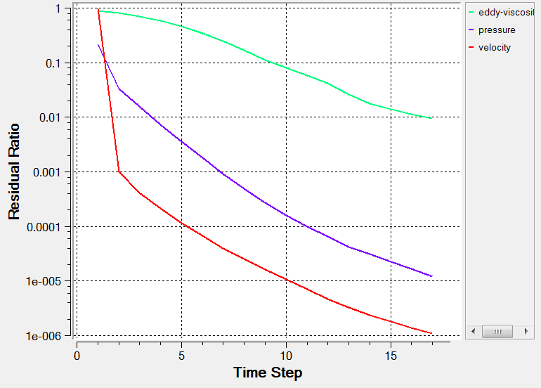
Figure 36. -
Click the User Function icon
 from the toolbar.
-
In the Function field of the User Function dialog, type
Fan_In = then paste the name you just copied.
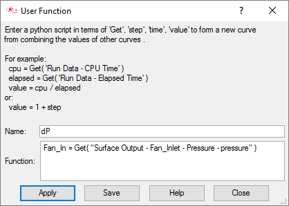
Figure 37. -
Paste the name in the Function field.
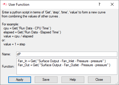
Figure 38. -
Type value = Fan_Out - Fan_In on a new line.
Note: The word “value” is case sensitive and should always be in lower case. If you use a capital letter, an error window appears.
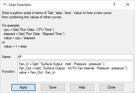
Figure 39. -
Click Apply.
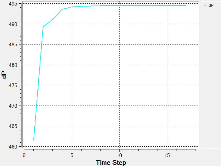
Figure 40.From the above figure, you can see the pressure rise got stabilized at around 9th iteration and remains constant with a pressure of 494.53 Pa for a given volume flow rate of 525.35 m3/hr which is very near compared to reference value of 494.91 Pa.
Summary
In this AcuSolve tutorial, you successfully set up and solved a problem involving the FAN_COMPONENT feature for an axial fan. The FAN_COMPONENT directly computes body force term to yield the pressure rise within the volume of interest. The problem simulated is the flow inside pipe with a fan placed at the middle of the pipe causing pressure rise due to fan and exits at the outlet. You started the tutorial by creating a database in AcuConsole, importing and meshing the geometry, and setting up the simulation parameters. The fluid domain is divided into three volumes – UpstreamDuct, Fan & DownstreamDuct – using the Volume Manager Dialog option. Once the case was setup, the solution was generated with AcuSolve. Results were plotted in AcuProbe by creating a user function to check for the fan pressure rise based on Fan_Inlet and Fan_Outlet pressures. New features that were introduced in this tutorial include: using Fan Component feature and explaining how the axial coefficients are calculated based on volume flow rate and fan pressure rise and using the User Function option in AcuProbe.