ACU-T: 5001 Blower - Transient (Sliding Mesh)
This tutorial provides the instructions for setting up, solving and viewing results for a transient simulation of a centrifugal air blower utilizing the sliding mesh approach. In this simulation, AcuSolve is used to compute and visualize the motion of fluid in form of velocity field, streamlines and particle path animations for three revolutions after the blower has been operating for a long time. This tutorial is designed to introduce you to a number of modeling concepts necessary to perform simulations that use the sliding mesh motion feature.
- Mesh motion
- Use of multiplier function to scale the time step size
- Assigning and meshing interface surfaces
- Mesh refinement
- Projection of steady state solution as the initial condition
- Post-processing using AcuFieldView to get velocity fields, streamlines and streaklines animation.
Prerequisites
In order to run this tutorial, you should have already run through ACU-T: 5000 Blower - Steady (Rotating Frame) and kept the solution in your working directory. It is assumed that you have some familiarity with AcuConsole, AcuSolve, and AcuFieldView. You will also need access to a licensed version of AcuSolve.
In case you do not have the steady state results, prior to running through this tutorial, copy AcuConsole_tutorial_input.zip from <AcuSolve installation directory>\model_files\tutorials\AcuSolve to a working directory and extract Centrifugal_Blower_MRF_Steady.acs from AcuConsole_tutorial_inputs.zip.
Analyze the Problem
The problem to be addressed in this tutorial is shown schematically in Figure 1 and Figure 2. It consists of a centrifugal blower with backward curved blades.

Figure 1. Schematic of Centrifugal Blower
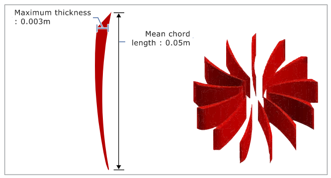
Figure 2. Schematic of Fan Blades
To capture the dynamic motion of the impeller blades, the simulation has to be run as transient. The converged steady state solution from the steady blower simulation is projected on the mesh and used as the initial state for the transient simulation.
The simulation will be run to model 0.12 s of the flow, which would constitute three revolutions of the fan blades with time step sizes scaled using a multiplier function.
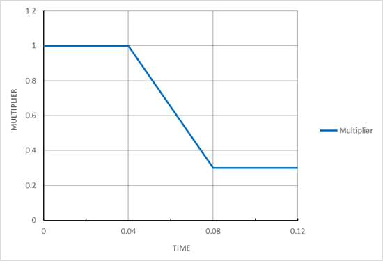
Figure 3.
The time step size for the last revolution is based on prior investigations of a similar geometry, which indicate that this time step size is small enough to capture the transient behavior of the flow. It should be noted, however, that a time step size sensitivity study should always be performed to establish appropriate time step size when analyzing a new application.
The CFD analysis of this problem offers detailed information about the flow through a centrifugal blower. To investigate this behavior, it is necessary to select an appropriate set of boundary conditions to use. There are two different methods that are commonly used. One approach is to specify the mass flow rate at the inlet of the blower and allow AcuSolve to compute the pressure drop, that is, flow forces simulation. Another option is to specify the stagnation pressure at the inlet and allow AcuSolve to compute the flow rate that results from this specified pressure change between the inlet and outlet. The boundary conditions used in this example are the latter. That is, the inlet is taken as stagnation pressure rather than mass flow rate so that AcuSolve calculates mass flow rates and pressure rise based on impeller rotation.
The fluid in this problem is air, which has a density of 1.225 kg/m3 and a viscosity of 1.781 X 10⁻⁵ kg/m-s.
In addition to setting appropriate conditions for the simulation, it is important to generate a mesh that will be sufficiently refined to provide good results. For this problem the global mesh size is set to provide approximately 16 elements around the circumference of the inlet which results in a mesh size of 0.02 m.
Note that higher mesh densities are required where velocity, pressure, and eddy viscosity gradients are larger. In this application, the flow will accelerate as it passes through radial flow paths between the fan blades. This leads to the higher gradients that need finer mesh resolution. Proper boundary layer parameters need to be set to keep the y+ near the wall surface to a reasonable level. The mesh density used in this tutorial is coarse and is intended to illustrate the process of setting up the model and to retain a reasonable run time. A significantly higher mesh density is needed to achieve a grid converged solution.
Once a solution is calculated, the flow properties of interest are the velocity magnitude, stream – lines and streak – lines animations as the blower goes through three revolutions of the impeller blades.
Define the Simulation Parameters
Start AcuConsole and Create the Simulation Database
In the next steps you will start AcuConsole, and open a database that is set up for a steady state simulation for the centrifugal blower using a rotating reference frame. You will then run AcuSolve to calculate a steady state solution, view the results with AcuFieldView, and save the database for the transient simulation.
-
Click and open Centrifugal_Blower_MRF_Steady.acs.
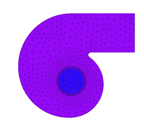
Figure 4. -
Run AcuSolve to solve the steady state problem.
-
Click
 on the toolbar to open the
Launch AcuSolve dialog.
Based on these settings, AcuConsole will generate the AcuSolve input files, then launch the solver. AcuSolve will run on four processors to calculate the steady state solution for this problem.
on the toolbar to open the
Launch AcuSolve dialog.
Based on these settings, AcuConsole will generate the AcuSolve input files, then launch the solver. AcuSolve will run on four processors to calculate the steady state solution for this problem. -
Click Ok to start the solution process.
While computing the solution, an AcuTail window opens. Solution progress is reported in this window. A summary of the solution process indicates that the run has been completed.
The information provided in the summary is based on the number of processors used by AcuSolve. If you use a different number of processors than indicated in this tutorial, the summary for your run may be slightly different than the summary shown.
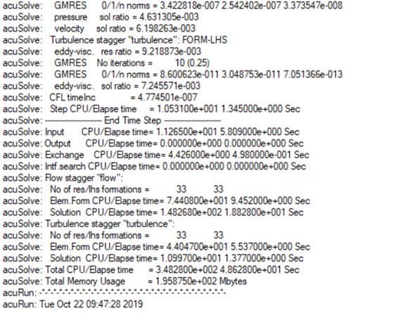
Figure 5.
-
Click
View Steady State Results
Set General Simulation Parameters
In next steps you will set parameters that apply globally to the simulation. To make this simple, the basic settings applicable for any simulation can be filtered using the BAS filter in the Data Tree Manager. This filter enables display of only a small subset of the available items in the Data Tree and makes navigation of the entries easier.
The general parameters that you will set for this tutorial are for turbulent flow, transient analysis, and mesh type as fully specified, which means that the motion is fully specified at the beginning of each time step and hence no mesh equation needs to be solved.
-
Click BAS in the Data Tree Manager to switch to basic view in the Data Tree.
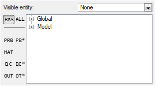
Figure 6. -
Double-click the Global
Data Tree item to expand it.
Tip: You can also expand a tree item by clicking
 next to the item name.
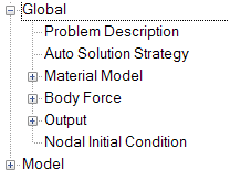
Figure 7. -
Set the Mesh type to Fully Specified.
This option indicates that the simulation will contain a moving mesh, but the motion of the mesh will be fully specified, that is, no differential equations will be solved to determine the deformation of the elements. Since the mesh is undergoing a simple rotational motion, this option provides the most efficient solution.
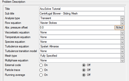
Figure 8.
Set Solution Strategy Parameters
In the next steps you will set attributes that control the behavior of AcuSolve as it progresses during the solution.
-
Set the Relaxation factor to 0.
The relaxation factor is used to improve convergence of the solution. The relaxation factor is used to improve convergence of the solution. Typically a value between 0.2 and 0.4 provides a good balance between achieving a smooth progression of the solution and the extra compute time needed to reach convergence. When solving transient solutions, the relaxation factor should be set to zero. A non-zero relaxation factor causes incremental updates of the solution, which will impact the time accuracy of the solution for transient cases.
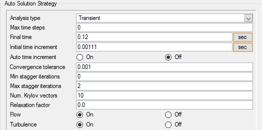
Figure 9.
Create a Multiplier Function for the Time Increment
AcuSolve provides the ability to scale values as a function of time and/or time step during a simulation. This is achieved through the use of a multiplier function. In this tutorial, the time steps sizes are scaled against time to set up a robust solution.
In the next steps you will create a multiplier function for the time increment. The multiplier function is chosen such that the impeller blades rotate at 10 degrees per time step for the first revolution (0 s– 0.04 s), then ramp down from 10 degrees per time step to 3 degrees per time step during the second revolution (0.04 s – 0.08 s) and complete the third revolution at 3 degrees per time step (0.08 s – .12 s)
To make the creation of the multiplier functions as simple as possible, you will use the PB* filter in the Data Tree Manager.
-
Set the Type to Piecewise Linear.
This option indicates that you will enter an array of numbers that will be used by AcuSolve to interpolate the value of the multiplier function at each time step. In this example, the curve fit is a function of time.
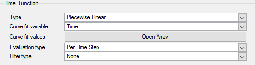
Figure 10. -
Add the curve-fit values for the large inlet temperature profile.
-
Enter the values shown as calculated earlier and shown in the following
image.
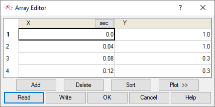
Figure 11.
-
Enter the values shown as calculated earlier and shown in the following
image.
-
Click Plot to expand the Array
Editor dialog to display the plot of the curve fit values.
Note: You may need to expand the dialog by dragging the right edge in order to see the plot.
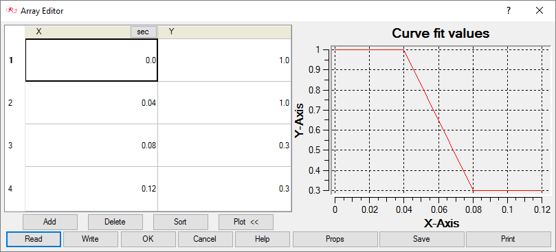
Figure 12.
Modify the Advanced Solution Strategy Parameters
AcuSolve provides additional features to modify some advanced solution strategy attributes separately, such as individual staggers (flow, mesh, turbulence, and so on), time increments, linear solver parameters and many more. In this tutorial the time increment feature is turned on in order to scale the time step sizes based on a multiplier function.
In the next steps you will work with the time increment feature under advanced solution strategy to assign the multiplier function.
-
In the Multiplier function drop-down menu, select
Time_Function.
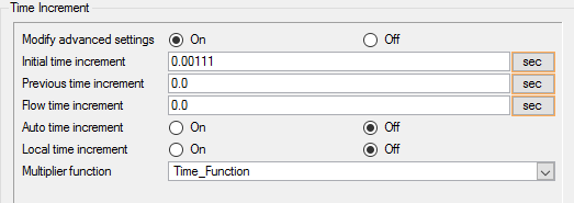
Figure 13.
Create the Mesh Motion
This command is used to simplify the specification of boundary conditions on mesh displacement and it can be used to simulate the dynamic motion of a rigid body. In this tutorial, the fluid region near the impeller blades is assigned a rotating mesh motion. The parameters defined for this would be the angular speed of the impeller blades and the center of rotation of the motion.
In the next steps you will create a mesh motion.
-
Set the Type to Rotation.
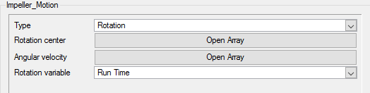
Figure 14.
Set the Nodal Output Frequency
The Nodal Output Frequency determines at what frequency or time interval the solution results would be stored to be used for post processing within AcuFieldView.
-
Set Output Initial Condition to On.
This writes the initial condition file.
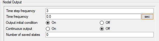
Figure 15.
Modify Volume Parameters
Volume groups are containers used for storing information about a volume region. This information includes solution and meshing parameters applied to the volume and the geometric regions that these settings are applied to.
-
Set the Reference frame as None.
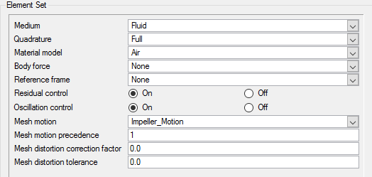
Figure 16.
Modify Surface Parameters
Surface groups are containers used for storing information about a surface, including solution and meshing parameters, and the corresponding surface in the geometry that the parameters will apply to.
- Fan Blades
- Interface
Modify Parameters for the Fan Blades
In the next steps you will specify the mesh motion associated with fan blades.
-
Set the Reference frame as None.
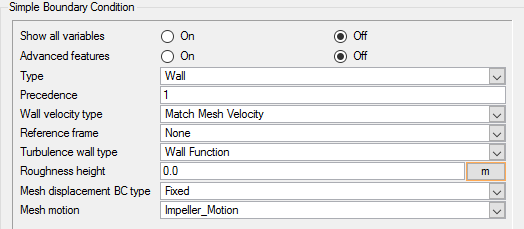
Figure 17.
Modify Parameters for the Interface
In the next steps you will assign Interface Surface properties to the Interface.
- Click ALE in the Data Tree Manager to see all the settings related to mesh motion.
- Expand Model, and then expand Surfaces.
-
Activate Interface Surface for Interface.
-
Set the Gap factor to 0.
Gap factor is non-dimensional (with respect to the length of an element face) maximum gap allowed for two element faces to be in contact.A gap factor of 0 means the maximum gap allowed is zero.
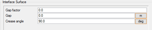
Figure 18.
-
Set the Gap factor to 0.
Assign Mesh Controls
Set Zone Meshing Attributes
In addition to setting meshing characteristics for the whole problem, you can assign meshing attributes to a zone within the problem where you want to be able to resolve flow with a mesh that is more refined than the global mesh. A zone mesh refinement can be created using basic shapes to control the mesh size within that shape. These types of mesh refinement are used when refinement is needed in an area that does not correspond to a geometric item.
In the following steps you will add mesh refinement in the zone around the impeller blades closest to the housing wall as shown in figure 3.
-
Set the location of the mesh refinement by defining the center points of the
end faces of the cylinder.
-
Enter the coordinate values as shown in the following image.
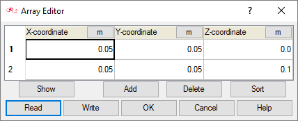
Figure 19.
-
Enter the coordinate values as shown in the following image.
-
Enter 0.005 m for the Mesh size.
This will result in a zone where the mesh size provides at least 10 cells between the impeller and the housing wall at their nearest distance.
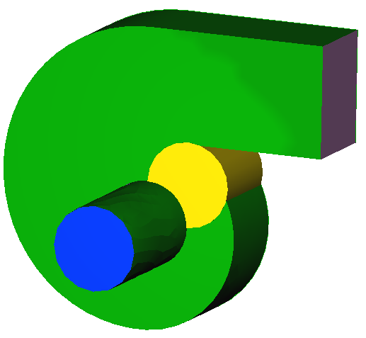
Figure 20.
Set Surface Meshing Parameters for the Interface
In the following steps you will set meshing attributes that will allow for localized control of the mesh size near on the interface.
-
Change the Boundary layer elements type to Mixed.
This is used to generate prism/hexahedral elements in the boundary layer.
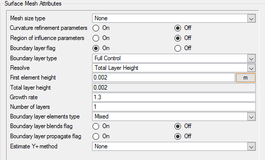
Figure 21.
Generate the Mesh
In the next steps you will generate the mesh that will be used when computing a solution for the problem.
-
Click
 on the toolbar to open the Launch
AcuMeshSim dialog.
For this case, the default settings will be used.
on the toolbar to open the Launch
AcuMeshSim dialog.
For this case, the default settings will be used. -
Click Ok to begin meshing.
During meshing an AcuTail window opens. Meshing progress is reported in this window. A summary of the meshing process indicates that the mesh has been generated.
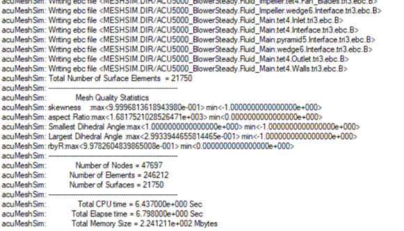
Figure 22.Note: The actual number of nodes and elements, and memory usage may vary slightly from machine to machine. -
Right-click on the model and select cut plane
visualization to view the mesh near the fan blades.
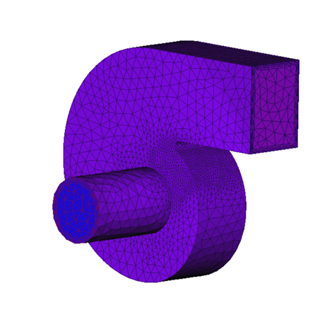
Figure 23. Mesh Details of the Geometry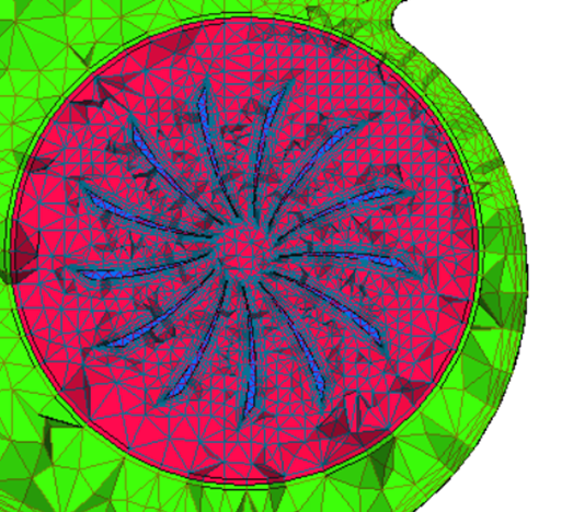
Figure 24. Mesh Details Near the Fan Blades
Split the Nodes on the Interface
At this point, the interface surface has one set of nodes which are either attached to the Fluid_Main or Fluid_Impeller volume sets. In order for the nodes inside the Fluid_Impeller volume and Interface to rotate based on the mesh motion prescribed, a duplicate set of nodes needs to be created, so that one set of the nodes follow the motion of the Fluid_Impeller and another set stays attached to Fluid_Main.
Splitting the nodes on the interface would allow the nodes attached to Fluid_Impeller to slide over the nodes on Fluid_Main, hence simulating the rotation on the fluid domain with the impeller blades.
In the next steps you will split the nodes on the interface using the Mesh Op. tool.
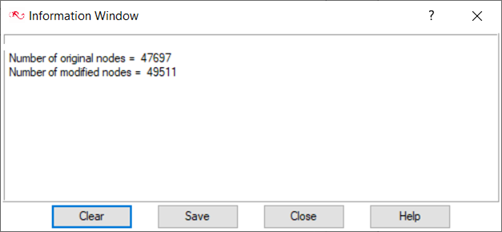
Figure 25.
Project Steady State Solution to Use as Initial Conditions
In the next steps you will use the Project Solution to project the steady state solution onto the transient case in form on Nodal Initial Conditions.
-
Browse to the location where the steady state solution is stored and select the
log file.
Once the log file is selected, the Information Window displays, showing the details of the projection process.
The AcuSolve solution projection dialog updates and displays the step ID and the variables to project.
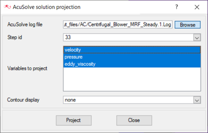
Figure 26. -
Click Open Array next to Nodal values for Pressure to
check that the values have been assigned.
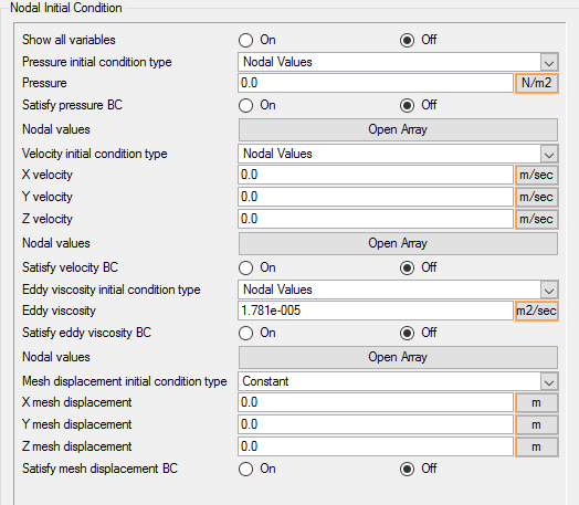
Figure 27.
Compute the Solution and Review the Results
Run AcuSolve
In the next steps you will launch AcuSolve to compute the solution for this case.
-
Click on the toolbar to open the
Launch AcuSolve dialog.
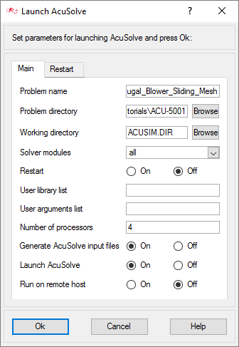
Figure 28.For this case, the default values will be used. AcuSolve will run using four processors and it will calculate the transient solution for this problem.
-
Click Ok to start the
solution process.
While computing the solution, an AcuTail window opens. Solution progress is reported in this window. A summary of the solution process indicates that the run has been completed.
The information provided in the summary is based on the number of processors used by AcuSolve. If you use a different number of processors than indicated in this tutorial, the summary for your run may be slightly different than the summary shown.
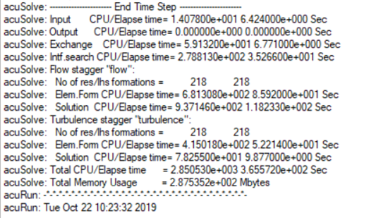
Figure 29.
View Transient Results with AcuFieldView
Now that a solution has been calculated, you are ready to view the flow field using AcuFieldView. AcuFieldView is a third-party post-processing tool that is tightly integrated to AcuSolve. AcuFieldView can be started directly from AcuConsole, or it can be started from the Start menu, or from a command line. In this tutorial you will start AcuFieldView from AcuConsole after the solution is calculated by AcuSolve.
In the following steps you will start AcuFieldView, display the pressure contours on the mid coordinate surface and generate animations for pressure, streamlines and particle paths.
Start AcuFieldView
-
Click
 on the
AcuConsole toolbar to open the
Launch AcuFieldView dialog.
on the
AcuConsole toolbar to open the
Launch AcuFieldView dialog.
-
Click Ok to start
AcuFieldView.
When you start AcuFieldView from AcuConsole, the results from the last time step of the solution that were written to disk will be loaded for post-processing. You will see that the pressure contours have already been displayed on all the boundary surfaces with mesh.
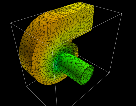
Figure 30.These steps are provided with the assumption that you are able to manipulate the view in AcuFieldView to have a white background, perspective turned off, outlines turned off, and the viewing direction set to +Z. If you are unfamiliar with basic AcuFieldView operations, refer to Manipulate the Model View in AcuFieldView.
Animate the Pressure Contours on the Mid Coordinate Surface
-
Click
 to open
the Coordinate Surface dialog.
to open
the Coordinate Surface dialog.
-
Activate the Frame check box to display the frame for the
legend.
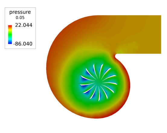
Figure 31. -
In the Flipbook Controls dialog, click on
Speed to open the Minimum Time Between
Frames dialog.
Figure 32.
Set up Streamlines
-
Click to open
the Coordinate Surface dialog.
-
Click
 to open the Boundary
Surface dialog.
to open the Boundary
Surface dialog.
-
Click the Mode toggle button and select Seed
a Surface.
In order to display streamlines you will need to seed a surface from where the streamlines are generated.
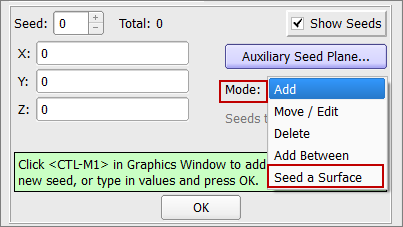
Figure 33. -
Ctrl + left click to select boundary surface 3
(Fan_Blades) as the surface to be seeded and click
OK.
The seeds are displayed on the fan blades.
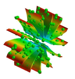
Figure 34. -
Change the Direction to Both.
The direction determines the direction of flow (upstream, downstream or both) in which the streamlines would be generated from the surface selected.
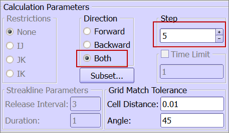
Figure 35. -
Click Calculate to generate the streamlines.
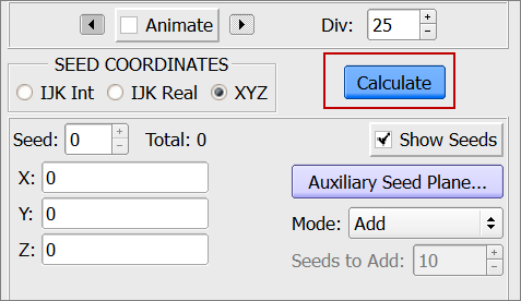
Figure 36. -
Orient the geometry so that all the surfaces are visible, as shown below:
Figure 37. -
In the Steamlines panel, click Animate to see the
streamlines.
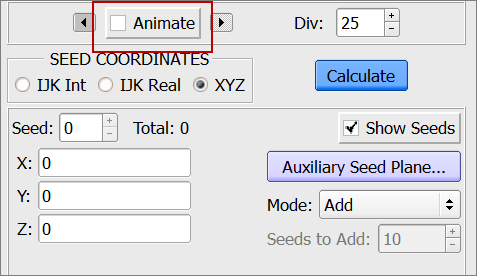
Figure 38.
Set up Streaklines
-
Pause the animation and click Save to save the
animation.
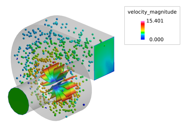
Figure 39.
Summary
In this tutorial, you worked through a basic workflow to set up a transient simulation with a sliding mesh in a centrifugal blower. Once the case was set up, you modified the mesh to include refinement zones, projected the steady state solution onto the refined mesh and generated a solution using AcuSolve.
Results were post-processed in AcuFieldView to allow you to create contour views for the pressure on the mid coordinate surface of the blower as well as the impeller blades along with new features for creating animations for contours, streamlines, streaklines and particle paths.
New features introduced in this tutorial include creating a rotational mesh motion, use of interface surfaces, projection of steady state solution in form of nodal initial conditions, creating pressure, streamlines and particle path animations.