ACU-T: 4200 Humidity – Pipe Junction
Prerequisites
This tutorial provides the instructions for setting up and running a basic transient humidity transport simulation using a pipe junction model. Prior to starting this tutorial, you should have already run through the introductory HyperWorks tutorial, ACU-T: 1000 HyperWorks UI Introduction, and have a basic understanding of HyperWorks CFD and AcuSolve. To run this simulation, you will need access to a licensed version of HyperWorks CFD and AcuSolve.
Prior to running through this tutorial, copy HyperWorksCFD_tutorial_inputs.zip from <Altair_installation_directory>\hwcfdsolvers\acusolve\win64\model_files\tutorials\AcuSolve to a local directory. Extract ACU-T4200_Humidity.hm from HyperWorksCFD_tutorial_inputs.zip.
Problem Description
The problem to be addressed in this tutorial is shown schematically in Figure 1. As an example, a pipe junction problem is attached here to show the capability of the Humidity modelling in AcuSolve. In this problem, there are two inlets with different flow, thermal, and humidity conditions. As the flow proceeds downstream of the pipe, two pipes merge into a single pipe to create a single outlet and a distinct profile of temperature and humidity is attained. The geometry is symmetric about the XZ midplane of the pipe, as shown in the figure.
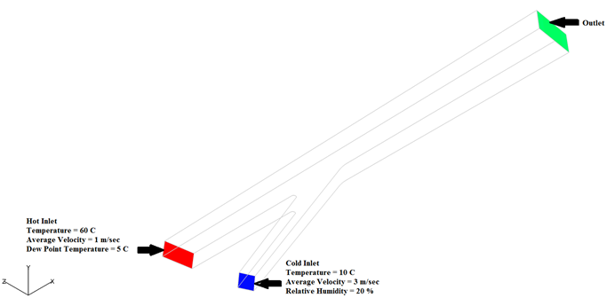
Figure 1.
Start HyperWorks CFD and Open the HyperMesh Database
-
From the Home tools, Files tool group, click the Open Model tool.

Figure 2.The Open File dialog opens.
Validate the Geometry
The Validate tool scans through the entire model, performs checks on the surfaces and solids, and flags any defects in the geometry, such as free edges, closed shells, intersections, duplicates, and slivers.
Figure 3.
Set Up Flow
Set Up the Simulation Parameters and Solver Settings
-
From the Flow ribbon, click the Physics tool.

Figure 4.The Setup dialog opens. -
Under the Physics models setting:
- Select the Multiphase flow radio button.
- Set the Multifluid type to Humidity transport.
- Set the Time step size to 1 s and the Final time to 50 s.
- Set the Turbulence model to Spalart-Allmaras.
- Set the Gravity to (0,-9.81,0).
-
Set the Pressure scale to Gauge and click
 . In the microdialog, set the Absolute pressure offset to 101325 Pa
then press Esc.
. In the microdialog, set the Absolute pressure offset to 101325 Pa
then press Esc.
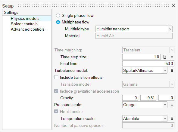
Figure 5. -
Set both the Minimum and Maximum stagger iterations to
2.
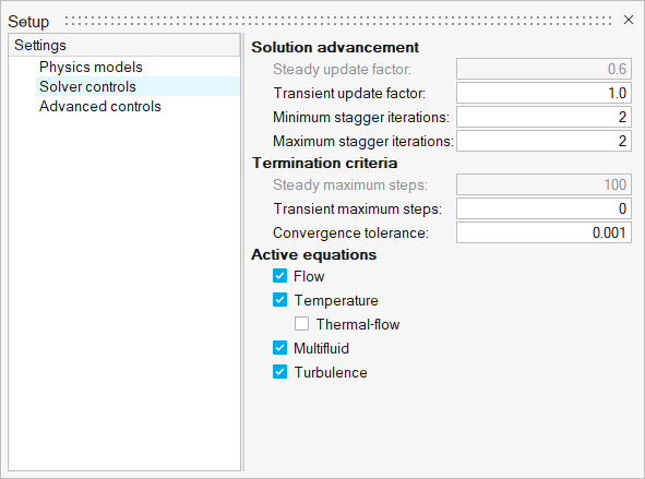
Figure 6.
Define Flow Boundary Conditions
-
From the Flow ribbon, Profiled
tool group, click the Profiled Inlet tool.

Figure 7. -
In the microdialog:
- Set the Average velocity to 1 m/sec.
- Set the Temperature to 333.15 K.
- Set the Humidity input type to Dewpoint Temperature.
- Set the Dewpoint temperature to 278.15 K.
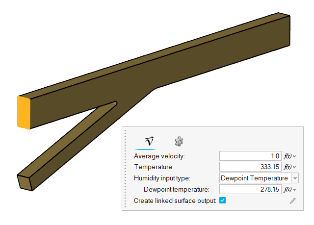
Figure 8. -
On the guide bar, click
 to execute the command and remain in the
tool.
to execute the command and remain in the
tool.
-
In the microdialog:
- Set the Average velocity to 3 m/sec.
- Set the Temperature to 283.15 K.
- Set the Humidity input type to Relative Humidity.
- Set the Relative humidity to 20.
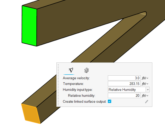
Figure 9. -
On the guide bar, click
 to execute
the command and exit the tool.
to execute
the command and exit the tool.
-
Click the Outlet tool.

Figure 10. -
Select the surface highlighted in the figure below then click
 on the
guide bar.
on the
guide bar.
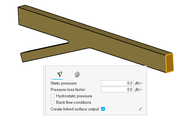
Figure 11. -
Click the Slip tool.

Figure 12. -
Select the surface highlighted in the figure below (the surface with the
minimum y-coordinate).
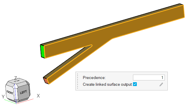
Figure 13. -
Click
 on the guide bar.
-
Select the surface highlighted in the figure below (the surface with the
maximum y-coordinate).
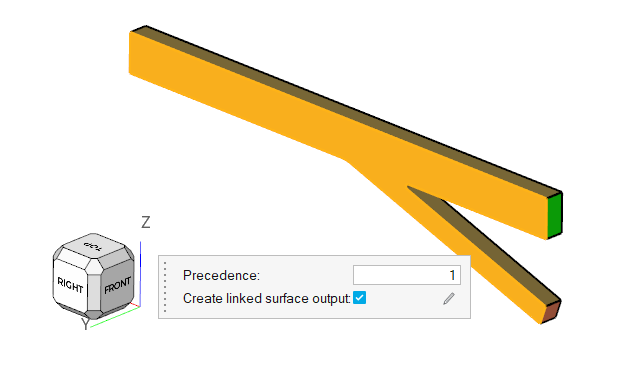
Figure 14. -
Click on the guide bar.
Compute the Solution
The input HyperMesh database contains the mesh, hence you do not need to generate the mesh again.
Define the Nodal Initial Conditions
-
From the Solution ribbon, click the Part tool.

Figure 15. -
In the dialog, click
 , select Relative Humidity
and Temperature from the list of variables, then click on
the white space in the dialog.
, select Relative Humidity
and Temperature from the list of variables, then click on
the white space in the dialog.
-
Set the initial values of Relative Humidity and Temperature to
20 and 333.15 K,
respectively
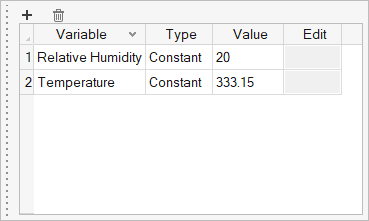
Figure 16. -
Click on the guide bar.
Run AcuSolve
-
From the Solution ribbon, click the Run tool.

Figure 17. -
Click Run to launch AcuSolve.
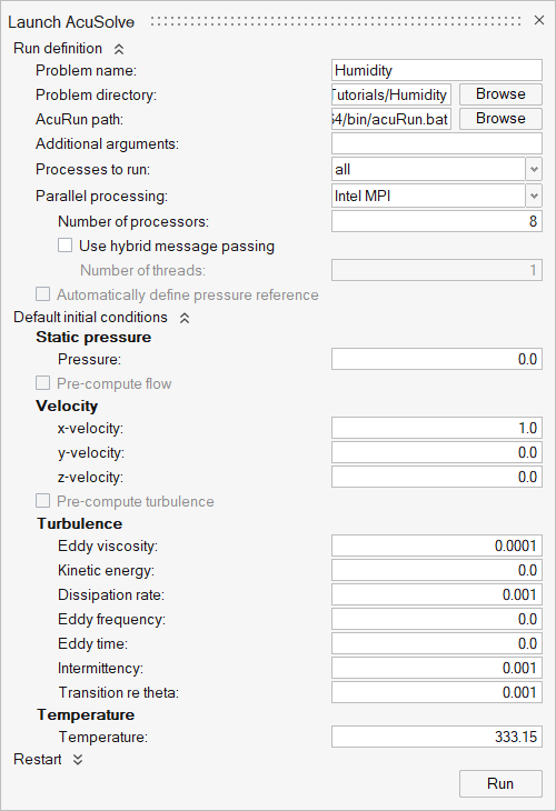
Figure 18.Tip: While AcuSolve is running, right-click on the AcuSolve job in the Run Status dialog and select View Log File to monitor the solution process. -
Click the Plot tool.

Figure 19. -
In the Plot Utility dialog, double-click on
Residual Ratio to plot the residuals.
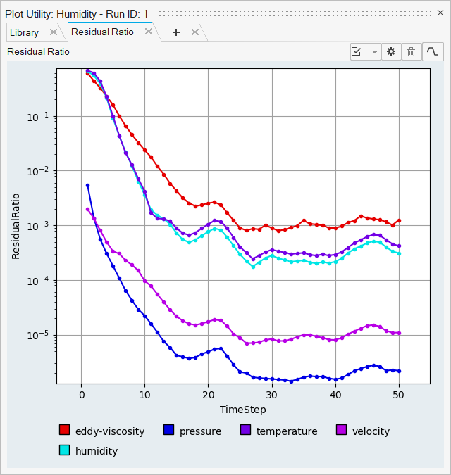
Figure 20.
Post-Process the Results with HW-CFD Post
In this step, you will create contour plots for temperature, relative humidity, mass fraction humidity, and velocity.
-
In the Post Browser, click on the icon beside
Flow Boundaries to turn off the display of all the
surfaces.
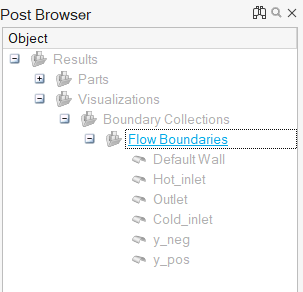
Figure 21. -
Click the Slice Planes tool.

Figure 22. -
Select the x-z plane in the modeling window.
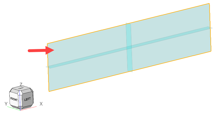
Figure 23. -
In the slice plane microdialog, click
 to
create the slice plane.
to
create the slice plane.
-
Click
 then activate the Legend
toggle.
then activate the Legend
toggle.
-
Click
 and set the Colormap Name to Rainbow
Uniform.
and set the Colormap Name to Rainbow
Uniform.
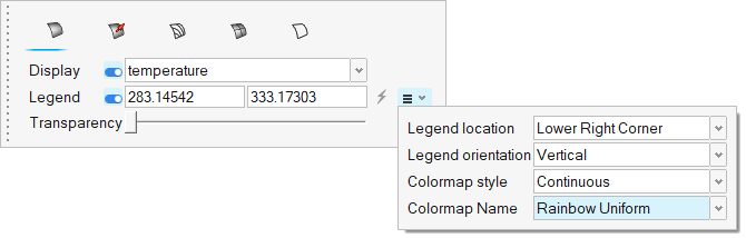
Figure 24. -
On the guide bar, click to
create the temperature contour plot.
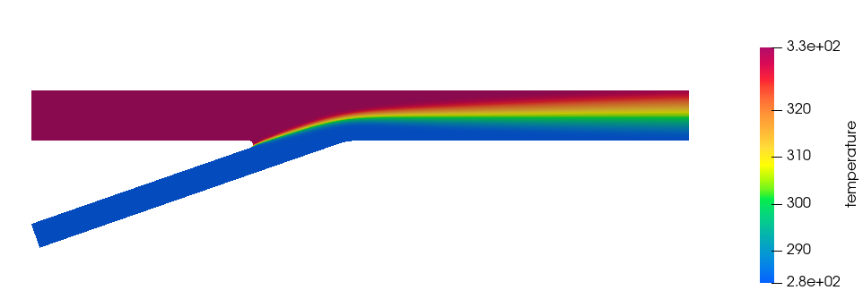
Figure 25. -
Hide the temperature contour and repeat the steps 5-11 to create a similar
contour plot for relative humidity.
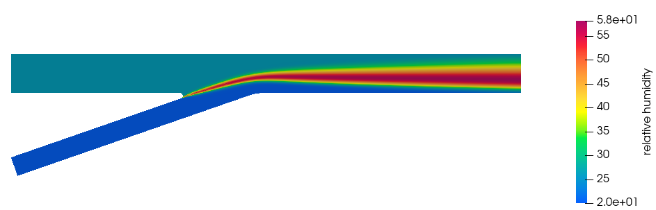
Figure 26. -
Hide the relative humidity contour and repeat the steps 5-11 to create a
similar contour plot for mass fraction humidity.
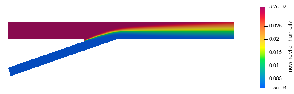
Figure 27. -
Hide the mass fraction humidity contour and repeat the steps 5-11 to create a
similar contour plot for velocity.
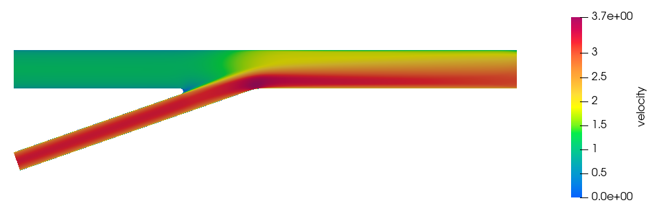
Figure 28.
Summary
In this tutorial, you learned how to set up and solve a humidity transport simulation using HyperWorks CFD and AcuSolve. You started by importing the HyperWorks CFD input database and then defined the flow setup. Once the solution was computed, you created a plot of residual ratios using the plot utility in HyperWorks CFD. Finally, you created a contour plot of temperature distribution, relative humidity, humidity mass fraction, and velocity using HyperWorks CFD Post.