ACU-T: 4002 Sloshing of Water in a Tank
Prerequisites
This tutorial provides instructions for running a transient simulation of a two-phase flow in a rectangular tank using the level set model. Prior to starting this tutorial, you should have already run through the introductory HyperWorks tutorial, ACU-T: 1000 HyperWorks UI Introduction, and have a basic understanding of HyperMesh, AcuSolve, and HyperView. To run this simulation, you will need access to a licensed version of HyperMesh and AcuSolve.
Prior to running through this tutorial, copy HyperMesh_tutorial_inputs.zip from <Altair_installation_directory>\hwcfdsolvers\acusolve\win64\model_files\tutorials\AcuSolve to a local directory. Extract ACU-T4002_SloshingTank.hm and gravity.c from HyperMesh_tutorial_inputs.zip.
Since the HyperMesh database (.hm file) contains meshed geometry, this tutorial does not include steps related to geometry import and mesh generation.
Problem Description
The problem to be solved is shown schematically in the figure below. It consists of a partially filled water tank and from time t=0, water inside the tank is subjected to a sinusoidal varying body force along x-direction and constant gravity along y-direction.

Figure 1.
The body force in the x-direction is given by the expression:
- Α = Amplitude of oscillation = -0.06 m
- ω = Frequency of oscillation = = 3.6 rad/sec
- T = Time period of oscillation = 1.74 sec
- φ = Phase difference = 0
Open the HyperMesh Model Database
-
Click the Open Model icon
 located on the standard toolbar.
The Open Model dialog opens.
located on the standard toolbar.
The Open Model dialog opens.
Set the General Simulation Parameters
Set the Analysis Parameters
-
Set the Multiphase equation to Level Set.
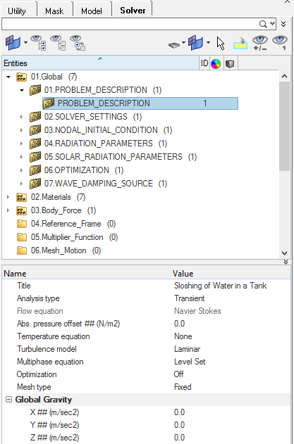
Figure 2. -
Check that the Flow and Field options are turned On.
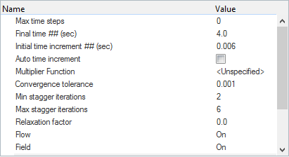
Figure 3.
Define the Nodal Outputs
- In the Solver Browser, expand 17.Output and click NODAL_OUTPUT.
- Set the Time step frequency to 10.
- Toggle On the Output initial condition field.
Create a Multiphase Model and Set the Body Force
Create a Multiphase Material Model
-
Enter Water as the Field 2 name.
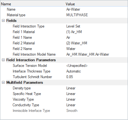
Figure 4.
Set the Body Force
-
Set the Number of user values to 3.
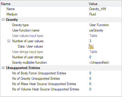
Figure 5. -
Enter (-0.06, 1.74, 0) as the three values then click
Close.
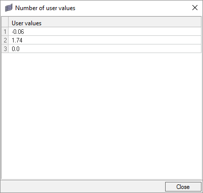
Figure 6.
Set the Boundary Conditions and Nodal Initial Conditions
Set the Boundary Conditions
-
Click Fluid. In the Entity Editor,
- Change the Type to MULTIPHASE
- Select Air-Water as the Material.
- Select Gravity_HM as the Body force.
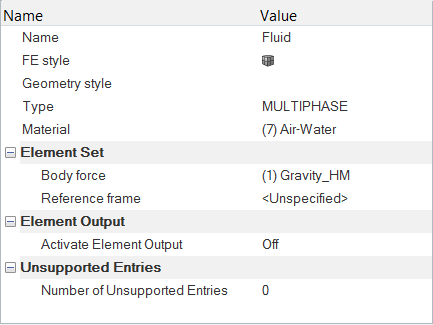
Figure 7. -
Click Wall. In the Entity Editor, verify that the Type is set to WALL.
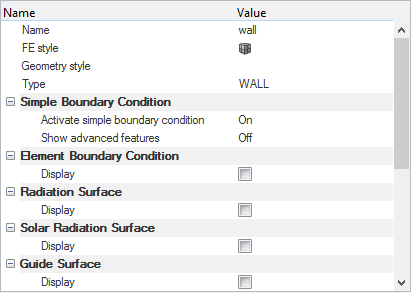
Figure 8. -
Change the Front and Rear
component Types to SLIP.
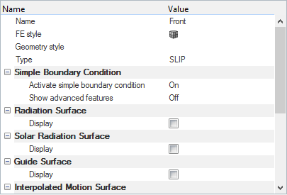
Figure 9.
Create a Node Set
- Go to the Model Browser, right-click on empty space in the browser area, and select .
- In the Entity Editor, rename the set to Water_Column.
Set the Nodal Initial Conditions
-
Set the Initial Volume Fraction to 1.0.
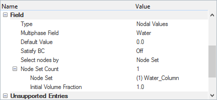
Figure 10.
Assign Nodes to the Node Set
-
Toggle on the Water_Column block then click
select.
All the nodes in the Water column block are highlighted in the graphics area.
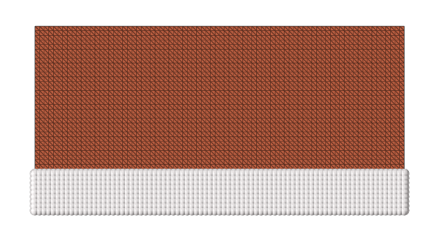
Figure 11.
Assign the Reference Pressure
-
Change the Boundary condition variable to
Pressure.
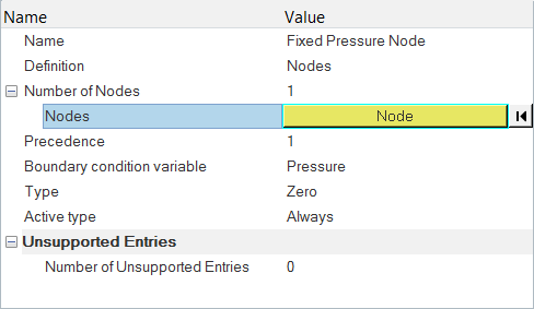
Figure 12.
Compute the Solution
In this step, you will launch AcuSolve directly from HyperMesh and compute the solution.
Run AcuSolve
-
Click
 on the ACU toolbar.
The Solver job Launcher dialog opens.
on the ACU toolbar.
The Solver job Launcher dialog opens. -
Leave the remaining options as
default and click Launch to start the solution
process.
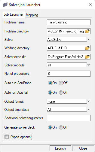
Figure 13.
Post-Process the Results with HyperView
Open HyperView and Load the Model and Results
-
In the Load model and results panel, click
 next
to Load model.
next
to Load model.
Create the Water Flow Animation
In this step, you will create an animation of the water flow as it fills in through the inlet.
-
Orient the display to the xy-plane by clicking
 on the Standard Views toolbar.
-
Click
 on the Results toolbar to open the Contour panel.
- Select Volume_fraction-2-Water (s) as the Result type.
- Click Apply to display the volume fraction contour at the first time step.
- Click the Legend tab then click Edit Legend.
- In the Edit Legend dialog, change the Number of levels to 2 and the Numeric format to Fixed.
-
On the Animation toolbar, click the Animation Controls icon
 .
.
- Drag the Max Frame Rate slider to 5 fps.
-
Click the Start/Pause Animation icon
 to play the animation in the graphics area.

Figure 14.
Save the Animation
-
On the ImageCapture toolbar, make sure that the Save Image to File option is
On.
-
Click the Capture Graphics Area Video icon
 .
The Save Graphics Area Video As dialog opens.
.
The Save Graphics Area Video As dialog opens.
Summary
In this tutorial, you successfully learned how to set up and solve a transient multiphase flow problem involving water sloshing in a tank using HyperMesh and AcuSolve. You also learned how to create a multiphase model using the Level Set method and specify the body force using a user-defined function and then compile the UDF. Once the solution was computed, you post-processed the results in HyperView where you generated an animation of the water sloshing in the tank.