ACU-T: 4001 Water Filling in a Tank
Prerequisites
This tutorial provides instructions for setting up, solving, and viewing results for a transient dam break simulation using the Level Set method. Prior to starting this tutorial, you should have already run through the introductory HyperWorks tutorial, ACU-T: 1000 HyperWorks UI Introduction, and have a basic understanding of HyperWorks CFD and AcuSolve. To run this simulation, you will need access to a licensed version of HyperWorks CFD and AcuSolve.
Prior to running through this tutorial, copy HyperWorksCFD_tutorial_inputs.zip from <Altair_installation_directory>\hwcfdsolvers\acusolve\win64\model_files\tutorials\AcuSolve to a local directory. Extract ACU-T4001_tank2D.x_t from HyperWorksCFD_tutorial_inputs.zip.
Problem Description
The problem to be solved is shown schematically in the figure below. It consists of a half-filled water tank at time t=0. Water is injected through the Inlet at t=0 and as the water fills in through the inlet, the water-air interface can be visualized in a transient simulation.

Figure 1.
Start HyperWorks CFD and Create the HyperMesh Model Database
-
Create a new .hm database in
one of the following ways:
- From the menu bar, click .
- From the Home tools, Files tool group, click the Save As tool.
Figure 2.
Import and Validate the Geometry
Import the Geometry
-
In the Geometry Import Options dialog, leave all the
default options unchanged then click Import.
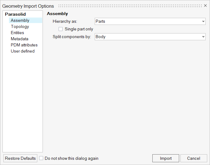
Figure 3.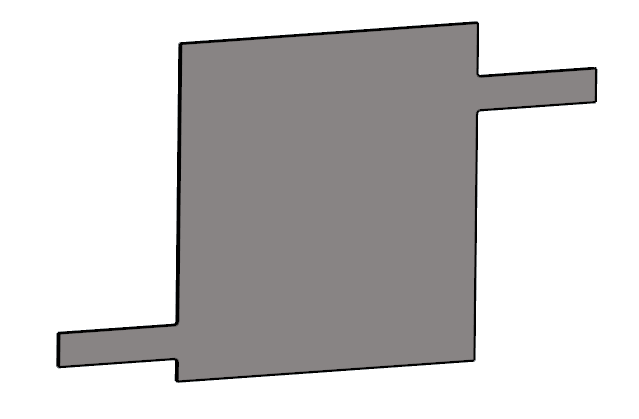
Figure 4.
Validate the Geometry
-
From the Geometry ribbon, click the Validate tool.

Figure 5.The Validate tool scans through the entire model, performs checks on the surfaces and solids, and flags any defects in the geometry, such as free edges, closed shells, intersections, duplicates, and slivers.The current model doesn’t have any of the issues mentioned above. Alternatively, if any issues are found, they are indicated by the number in the brackets adjacent to the tool name.
Observe that a blue check mark appears on the top-left corner of the Validate icon. This indicates that the tool found no issues with the geometry model.
Figure 6.
Set Up the Problem
Set Up the Simulation Parameters and Solver Settings
-
From the Flow ribbon, click the Physics tool.

Figure 7.The Setup dialog opens. -
Under the Physics models setting:
- Activate the Multiphase flow radio button.
- Set the Multifluid type to Immiscible and the Immiscible material to Air-Water
- Set the Time step size to 0.01 and the Final time to 3.0
- Select Laminar as the Turbulence model.
- Set the gravity to -9.81 m/sec2 in the y direction.
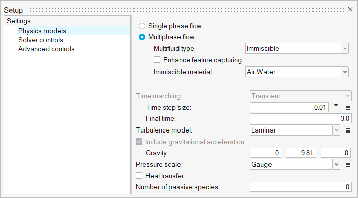
Figure 8. -
Click the Solver Controls setting and set the Maximum
stagger iterations to 4.
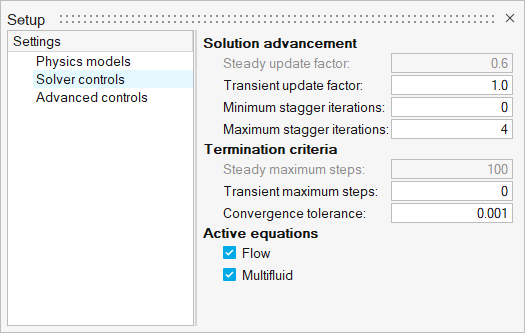
Figure 9.
Assign Material Properties
-
From the Flow ribbon, click the Material tool.

Figure 10. -
In the microdialog, select
Air-Water from the Material drop-down.
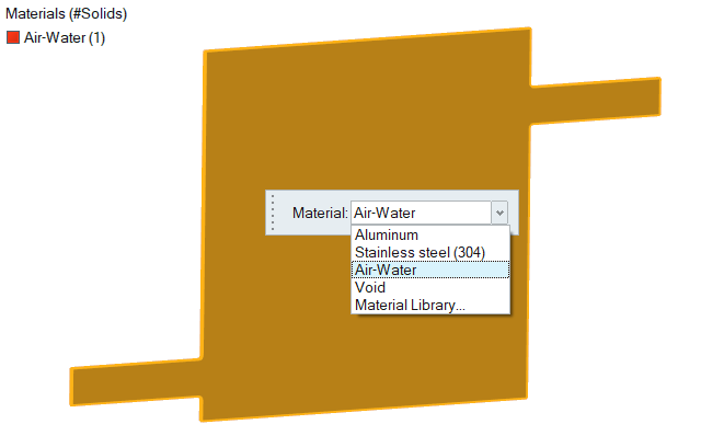
Figure 11. -
On the guide bar, click
 to execute
the command and exit the tool.
to execute
the command and exit the tool.
Define Flow Boundary Conditions
-
From the Flow ribbon, click the Slip tool.

Figure 12. -
Select the right most face on the positive z-axis, as shown in the figure
below.
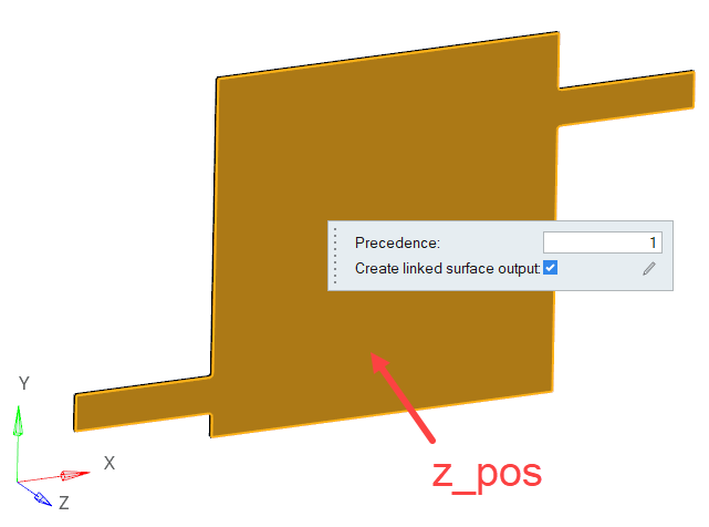
Figure 13. -
On the guide bar, click
 to execute the command and remain in the
tool.
to execute the command and remain in the
tool.
-
On the guide bar, click
to execute
the command and exit the tool.
-
Click the Constant tool.

Figure 14. -
Select the inlet surface shown in the figure below.
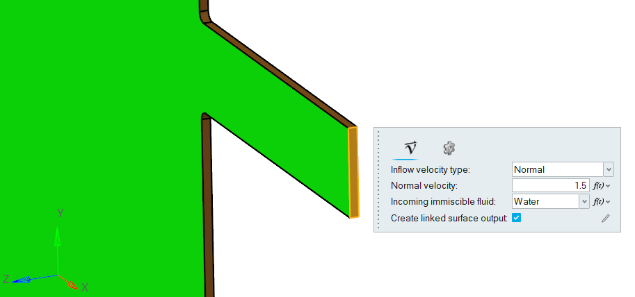
Figure 15. -
On the guide bar, click
to execute
the command and exit the tool.
-
Click the Outlet tool.

Figure 16. -
Select the outlet surface shown in the figure below.
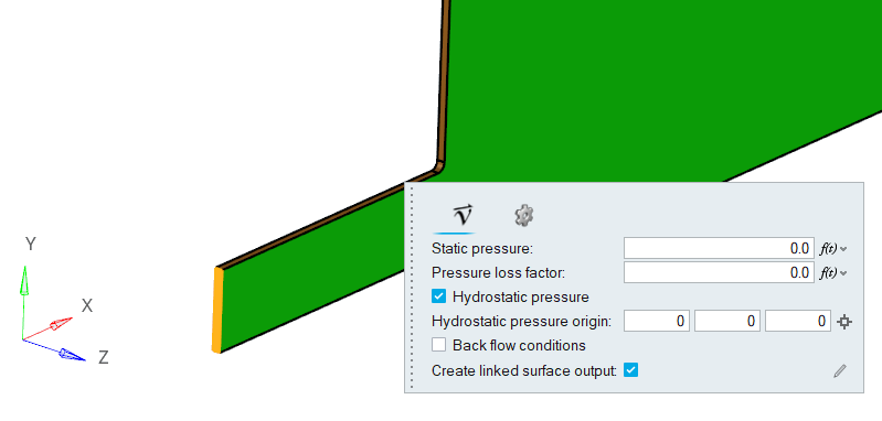
Figure 17. -
On the guide bar, click
to execute
the command and exit the tool.
Generate the Mesh
In this step, first you will create a surface mesh using the Interactive meshing tool; then, you will specify a global mesh size and growth rate for the model and generate the volume mesh using the Batch tool in the Mesh ribbon.
Create Surface Mesh
-
From the Mesh ribbon, click the Interactive tool.

Figure 18.By default, the Create should be selected from the secondary ribbon. -
Click
 on the guide bar to open the options menu, then make the following
changes:
on the guide bar to open the options menu, then make the following
changes:
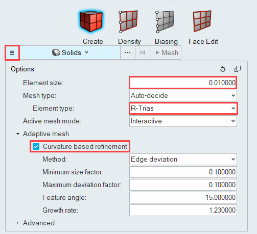
Figure 19.
Generate Volume Mesh
-
From the Mesh ribbon, click the
Volume tool.

Figure 20.The Meshing Operations dialog opens. -
Set the Mesh growth rate to 1.0.
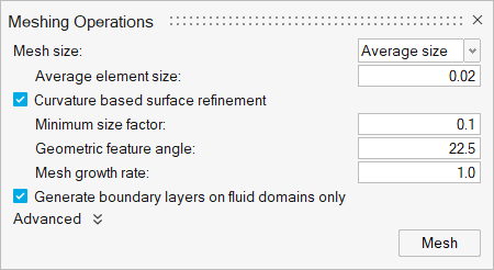
Figure 21.
Define Nodal Outputs and Nodal Initial Conditions
In this step, you will define the nodal output frequency and then specify the nodal initial conditions for the water column.
Define Nodal Output Frequency
-
From the Solution ribbon, click the Field tool.

Figure 22.The Field Output dialog opens. -
Set the Time step interval to 1.
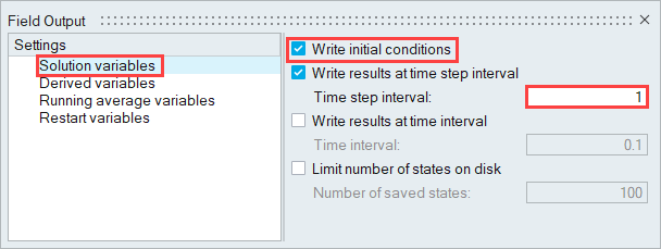
Figure 23.
Define the Nodal Initial Conditions
-
From the Solution ribbon, click the
Plane tool.

Figure 24. -
Click on the tank solid and verify the selection on the guide bar.

Figure 25. -
In the microdialog, click
 in
the top-left corner, select Fluid, then click in empty
space in the dialog.
in
the top-left corner, select Fluid, then click in empty
space in the dialog.
-
Change the Value field to Water.
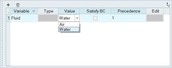
Figure 26. -
Click
 in the
top-right corner to orient the plane with the Vector
tool.
in the
top-right corner to orient the plane with the Vector
tool.
-
In the plane definition microdialog, verify that the
normal orientation is along the negative y-axis (i.e. 0, -1, 0).
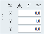
Figure 27. -
Click
 , set
the coordinates to (0, 0, 0), then press
Enter.
, set
the coordinates to (0, 0, 0), then press
Enter.
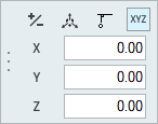
Figure 28. -
On the guide bar, click
to execute
the command and exit the tool.
Run AcuSolve
-
From the Solution ribbon, click the Run tool.

Figure 29.The Launch AcuSolve dialog opens. -
Leave the remaining options as default and click
Run to launch AcuSolve.
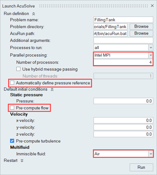
Figure 30.The Run Status dialog opens. Once the run is complete, the status is updated and you can close the dialog.Tip: While AcuSolve is running, right-click on the AcuSolve job in the Run Status dialog and select View Log File to monitor the solution process.
Post-Process the Results with HW-CFD Post
-
Click the Top face on the View Cube to align the
model.
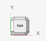
Figure 31. -
Activate the Legend toggle and click
 to refresh the range.
-
Click
 , set the Colormap style to
Filled, the Number of colors to
2, and the Colormap Name to Rainbow
Desaturated.
, set the Colormap style to
Filled, the Number of colors to
2, and the Colormap Name to Rainbow
Desaturated.
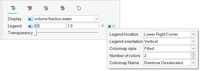
Figure 32. -
Click
 on the guide bar.
-
Click
 at the bottom of the modeling window to view a live animation of the flow.
Figure 33. -
Save the animation.
- Go to .
-
Click
 on the toolbar.
- Uncheck Include mouse cursor.
- Set the frame rate to 30.
-
Click
 on the toolbar then drag over the area you
want to record.
on the toolbar then drag over the area you
want to record.
-
Click
 to start recording and the same button to
stop recording.
to start recording and the same button to
stop recording.
- Name the file and save it.
Summary
In this tutorial, you successfully learned how to set up and solve a multiphase flow tank filling problem using HyperWorks CFD and AcuSolve. You started by importing the geometry and then completed the flow set up. Once the volume meshing was done, you specified the field initial conditions for the water column using the plane initialization tool. Once the solution was computed, you post-processed the results using the Post ribbon where you generated an animation of the water flow.