ACU-T: 4000 Transient Dam Break Simulation

Prerequisites

This tutorial introduces you to the workflow for setting up an AcuSolve transient dam break simulation using HyperWorks CFD. Prior to starting this tutorial, you should have already run through the introductory HyperWorks tutorial, ACU-T: 1000 HyperWorks UI Introduction, and have a basic understanding of HyperWorks CFD and AcuSolve. To run this simulation, you will need access to a licensed version of HyperWorks CFD and AcuSolve.

Prior to running through this tutorial, copy HyperWorksCFD_tutorial_inputs.zip from <Altair_installation_directory>\hwcfdsolvers\acusolve\win64\model_files\tutorials\AcuSolve to a local directory. Extract ACU-T4000_dambreak2D.x_t from HyperWorksCFD_tutorial_inputs.zip.

Problem Description

The problem to be addressed in this tutorial is shown schematically in the figure below. It consists of a square water column held in place by the reservoir walls. At time t=0, the walls are removed and the water column is now free to flow out. The simulation can be used to visualize and study the surge patterns as the column of water rushes out, as in a dam wall break.


Figure 1.

Start HyperWorks CFD and Create the HyperMesh Model Database

  1. Start HyperWorks CFD from the Windows Start menu by clicking Start > Altair <version> > HyperWorks CFD.
    When HyperWorks CFD is loaded, the Geometry ribbon is open by default.
  2. Create a new .hm database in one of the following ways:
    • From the menu bar, click File > Save.
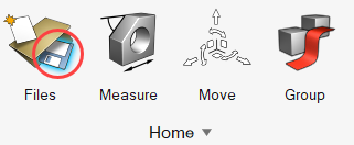
    • From the Home tools, Files tool group, click the Save As tool.


      Figure 2.
  3. In the Save File As dialog, navigate to the directory where you would like to save the database.
  4. Enter DamBreak as the name for the database then click Save.
    This will be your problem directory and all the files related to the simulation will be stored in this location.

Import and Validate the Geometry

Import the Geometry

  1. From the menu bar, click File > Import > Geometry Model.
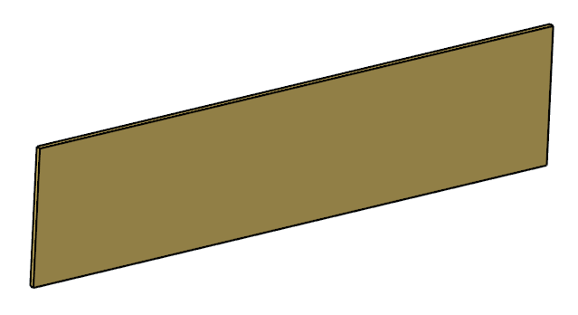
  2. In the Import File dialog, browse to your working directory then select ACU-T4000_dambreak2D.x_t and click Open.
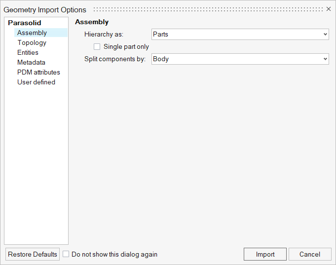
  3. In the Geometry Import Options dialog, leave all the default options unchanged then click Import.


    Figure 3.


    Figure 4.

Validate the Geometry

  1. From the Geometry ribbon, click the Validate tool.


    Figure 5.
    The Validate tool scans through the entire model, performs checks on the surfaces and solids, and flags any defects in the geometry, such as free edges, closed shells, intersections, duplicates, and slivers.

    The current model doesn’t have any of the issues mentioned above. Alternatively, if any issues are found, they are indicated by the number in the brackets adjacent to the tool name.

    Observe that a blue check mark appears on the top-left corner of the Validate icon. This indicates that the tool found no issues with the geometry model.


    Figure 6.
  2. Press Esc or right-click in the modeling window and swipe the cursor over the green check mark from right to left.
  3. Save the database.

Set Up the Problem

Set Up the Simulation Parameters and Solver Settings

  1. From the Flow ribbon, click the Physics tool.


    Figure 7.
    The Setup dialog opens.
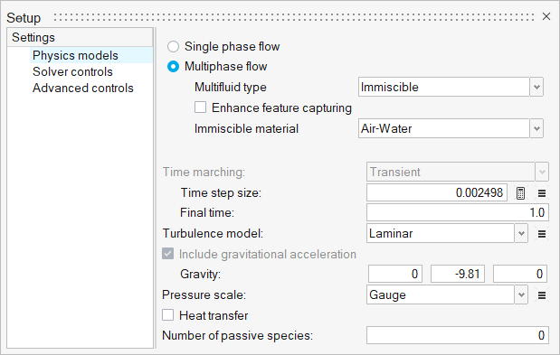
  2. Under the Physics models setting:
    1. Activate the Multiphase flow radio button.
    2. Set the Multifluid type to Immiscible and the Immiscible material to Air-Water
    3. Set the Time step size to 0.002498 and the Final time to 1.0
    4. Select Laminar as the Turbulence model.
    5. Set the gravity to -9.81 m/sec2 in the y direction.


    Figure 8.
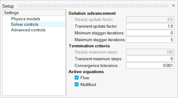
  3. Click the Solver Controls setting and set the Maximum stagger iterations to 5.


    Figure 9.
  4. Close the dialog and save the model.

Assign Material Properties

  1. From the Flow ribbon, click the Material tool.


    Figure 10.
  2. Click anywhere on the dam geometry.
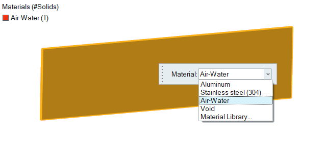
  3. In the microdialog, select Air-Water from the Material drop-down.


    Figure 11.
  4. On the guide bar, click to execute the command and exit the tool.
  5. Save the database.

Define Flow Boundary Conditions

  1. From the Flow ribbon, click the Symmetry tool.


    Figure 12.
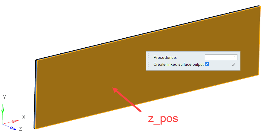
  2. Select the right most face on the positive z-axis, as shown in the figure below.


    Figure 13.
  3. In the Boundaries legend, double-click on Symmetry, rename it to z_pos and press Enter.
  4. On the guide bar, click to execute the command and remain in the tool.
  5. Rotate the model and select the opposite face.
  6. In the Boundaries legend, rename Symmetry to z_neg.
  7. On the guide bar, click to execute the command and exit the tool.
  8. Save the database.

Generate the Mesh

In this step, first you will create a surface mesh using the Interactive meshing tool; then, you will specify a global mesh size and growth rate for the model and generate the volume mesh using the Batch tool in the Mesh ribbon.

Create Surface Mesh

  1. From the Mesh ribbon, click the Interactive tool.


    Figure 14.
    By default, the Create should be selected from the secondary ribbon.
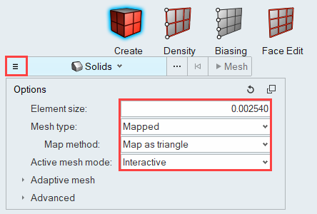
  2. Click on the guide bar to open the options menu, then make the following changes:
    1. Set the Element size to 0.00254.
    2. Set the Mesh type to Mapped.
    3. Set the Map method to Map as triangle.


    Figure 15.
  3. On the guide bar, change the entity selector to Solids then select the solid in the modeling window.
  4. Click Mesh in either the microdialog or on the guide bar to generate the surface mesh.
  5. Once the surface mesh is created, press Esc to exit out of the tool.

Generate Volume Mesh

  1. From the Mesh ribbon, click the Volume tool.


    Figure 16.
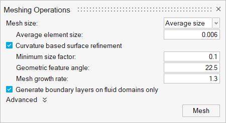
    The Meshing Operations dialog opens.
  2. Verify that the Mesh size option is set to Average size.
  3. Set the Average element size to 0.006.


    Figure 17.
  4. Click Mesh.
    The Run Status dialog opens. Once the run is complete, the status is updated and you can close the dialog.
    Tip: Right-click on the mesh job and select View log file to view a summary of the meshing process.

Define Nodal Outputs and Nodal Initial Conditions

In this step, you will define the nodal output frequency and then specify the nodal initial conditions for the water column.

Define Nodal Output Frequency

  1. From the Solution ribbon, click the Field tool.


    Figure 18.
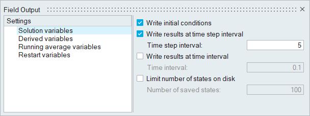
    The Field Output dialog opens.
  2. Click the Solution variables setting.
  3. Activate the Write initial conditions option.
  4. Verify that the Write results at time step interval option is active.
  5. Set the Time step interval to 5.


    Figure 19.

Define the Nodal Initial Conditions

  1. From the Solution ribbon, Zones tool group, click the Box tool.


    Figure 20.
  2. Hover the cursor over the dam geometry. When the zone is aligned with the surfaces of the model, double-click on the geometry.
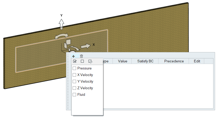
    An initialization zone with arbitrary dimensions should be visible on the model.


    Figure 21.
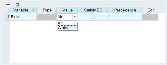
  3. In the microdialog, select Fluid then click in empty space in the dialog. Change the Value field to Water.


    Figure 22.
  4. In the zone initialization microdialog, expand the drop-down and set the dimensions of the zone as shown in the figure below.


    Figure 23.
    Note: If you do not see the microdialog for entering the dimensions, move the NIC variable microdialog.
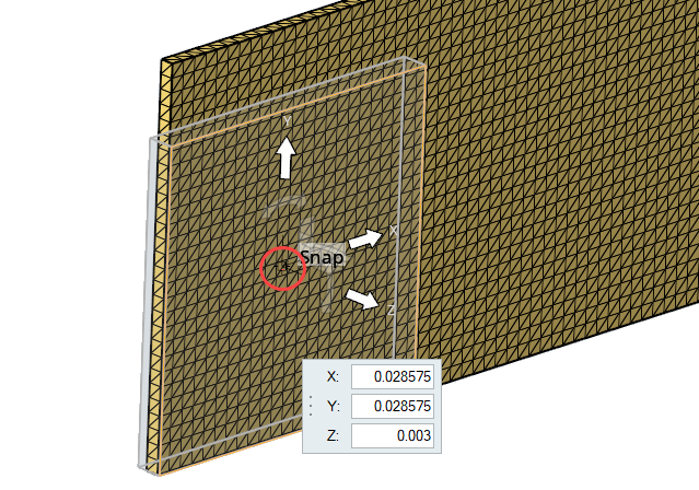
  5. Click the center of the manipulator on the model, as shown in the figure below, then enter the following coordinates for the center: 0.028575, 0.028575, 0.003.


    Figure 24.

    This will ensure that the fluid domain is initialized with a water column at the corner of the dam.

  6. Right-click in the modeling window and select the check mark to exit the tool.

Run AcuSolve

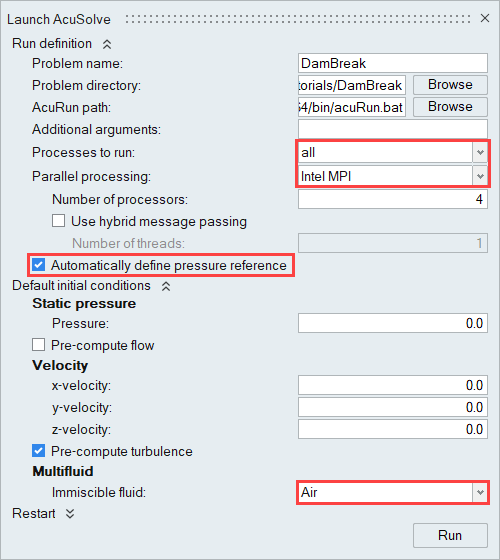
  1. From the Solution ribbon, click the Run tool.


    Figure 25.
    The Launch AcuSolve dialog opens.
  2. Set the Parallel processing option to Intel MPI.
  3. Optional: Set the number of processors to 4 or 8 based on availability.
  4. Verify that the Automatically define pressure reference option is active.
  5. Expand the Default initial conditions tab and deactivate the Pre-compute flow option.
  6. Set all the velocity components to 0 and set the Immiscible fluid to Air (if not already set).
  7. Leave the remaining options as default and click Run to launch AcuSolve.


    Figure 26.
    The Run Status dialog opens. Once the run is complete, the status is updated and you can close the dialog.
    Tip: While AcuSolve is running, right-click on the AcuSolve job in the Run Status dialog and select View Log File to monitor the solution process.

Post-Process the Results with HW-CFD Post

  1. Once the solution is completed, navigate to the Post ribbon.
  2. From the menu bar, click File > Open > Results.
  3. Select the AcuSolve log file in your problem directory to load the results for post-processing.
    The solid and all the surfaces are loaded in the Post Browser.
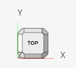
  4. Click the Top face on the View Cube to align the model.


    Figure 27.
  5. Right-click on the z_pos boundary in the Post Browser and select Edit.
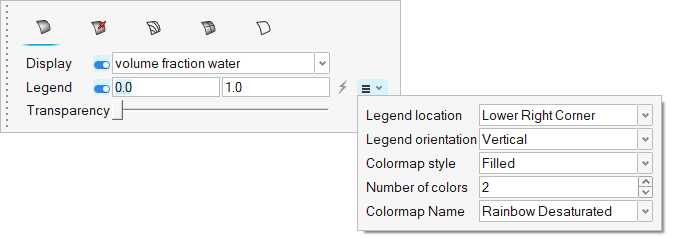
  6. In the display properties microdialog, set the display to volume fraction water.
  7. Activate the Legend toggle and click to refresh the range.
  8. Click , set the Colormap style to Filled, the Number of colors to 2, and the Colormap Name to Rainbow Desaturated.


    Figure 28.
  9. Click on the guide bar.
  10. Click at the bottom of the modeling window to view a live animation of the flow.


    Figure 29.
  11. Save the animation.
    1. Go to File > Screen Capture > Advanced Capture.
    2. Click on the toolbar.
    3. Uncheck Include mouse cursor.
    4. Set the frame rate to 30.
    5. Click on the toolbar then drag over the area you want to record.
    6. Click to start recording and the same button to stop recording.
    7. Name the file and save it.

Summary

In this tutorial, you successfully learned how to set up and solve a multiphase flow problem using HyperWorks CFD and AcuSolve. You started by importing the geometry and then completed the flow set up. Once the volume meshing was done, you specified the field initial conditions for the water column using the zone initialization tool. Once the solution was computed, you post-processed the results using the Post ribbon. Here, you generated an animation of the water flow as it surged once the dam walls were removed.