ACU-T: 3310 Single Phase Nucleate Boiling
This tutorial provides instructions for modeling a single-phase nucleate boiling using HyperWorks CFD. Prior to starting this tutorial, you should have already run through the introductory HyperWorks tutorial, ACU-T: 1000 HyperWorks UI Introduction, and have a basic understanding of HyperWorks CFD and AcuSolve. To run this simulation, you will need access to a licensed version of HyperWorks CFD and AcuSolve.
Prior to running through this tutorial, copy HyperWorksCFD_tutorial_inputs.zip from <Altair_installation_directory>\hwcfdsolvers\acusolve\win64\model_files\tutorials\AcuSolve to a local directory. Extract ACU-T3310_NB1_Steiner.hm from HyperWorksCFD_tutorial_inputs.zip.
Problem Description

Figure 1. Schematic of Channel
The dimensions of the inlet are 0.03 x 0.04 m; the inlet velocity (v) is 0.39 m/s and the temperature (T) of the fluid entering the inlets is 368.15 K (95 C).
The preheated air enters the inlets and heat is transferred to the fluid from the walls. The heat causes sub-cooled boiling to occur in the region close to the wall and leads to formation of bubbles at nucleation sites.
The heat transfer in this regime is basically dominated by two effects, the macro convection due to the motion of the bulk liquid and the latent heat transport associated with the evaporation of the liquid micro-layer between the bubble and the heated wall.
The fluid in this problem is water, which has temperature dependent material properties: density, viscosity, enthalpy and conductivity. There are also surface tension and vapor phase models specified for this material.
Water vapor which also has temperature dependent material properties is specified as the vapor phase model.
The AcuSolve simulation will be set up to model steady state heat transfer to determine the temperature and heat flux on the heated walls of the manifold.
Start HyperWorks CFD and Open the HyperMesh Database
-
From the Home tools, Files tool group, click the Open Model tool.

Figure 2.The Open File dialog opens.
Validate the Geometry
The Validate tool scans through the entire model, performs checks on the surfaces and solids, and flags any defects in the geometry, such as free edges, closed shells, intersections, duplicates, and slivers.
Figure 3.
Set Up Flow
Set the General Simulation Parameters
-
From the Flow ribbon, click the Physics tool.

Figure 4.The Setup dialog opens. -
Under the Physics models setting:
- Verify that Time marching is set to Steady.
- Select Spalart-Allmaras as the Turbulence model.
- Activate the Heat transfer checkbox.
- Click the Solve for boiling checkbox to activate Nucleate Boiling.
- Select Vapor_Therm for the Vapor phase model.
- Check that the Surface tension type is set to Constant and set the Surface tension value to 0.01.
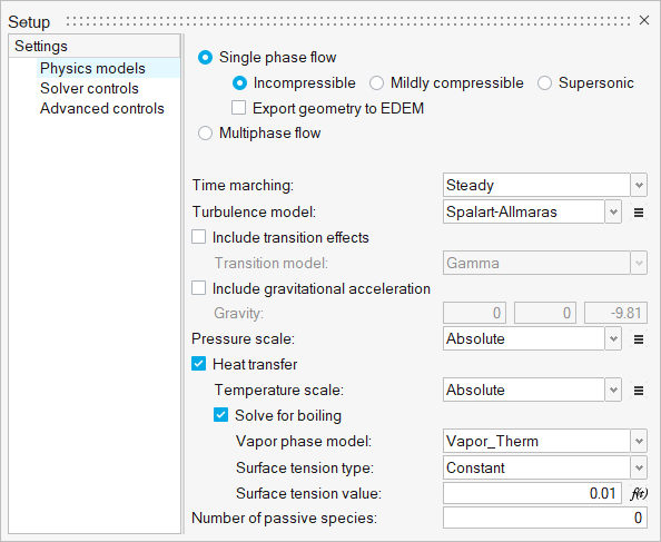
Figure 5.
Assign Material Properties
-
From the Flow ribbon, click the Material tool.

Figure 6. -
Select Water_Therm from the Material drop-down
menu.
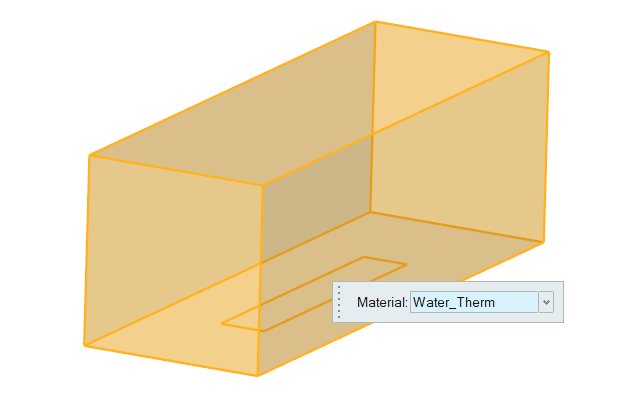
Figure 7. -
On the guide bar, click
 to execute
the command and exit the tool.
to execute
the command and exit the tool.
Define Flow Boundary Conditions
-
From the Flow ribbon, Profiled
tool group, click the Profiled Inlet tool.

Figure 8. -
In the microdialog, enter 0.39
for the Average velocity and 368.15 for the
Temperature.
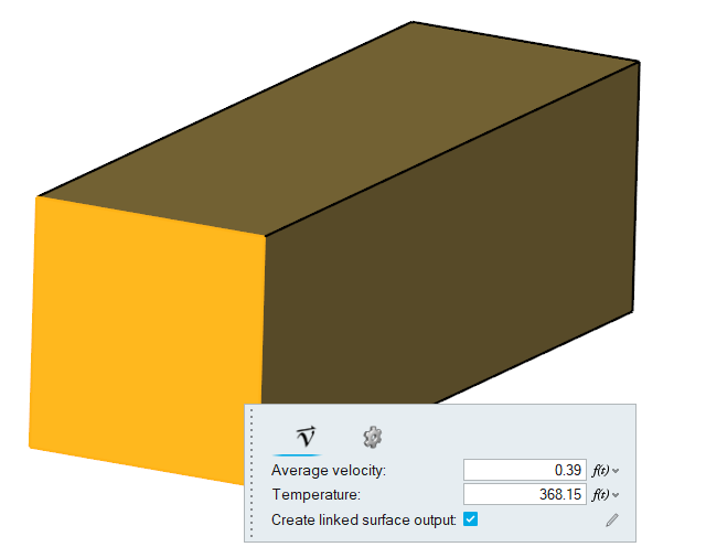
Figure 9. -
On the guide bar, click
to execute
the command and exit the tool.
-
Click the Outlet tool.

Figure 10. -
Select the face highlighted in the figure below, set the Static pressure to
200000, and activate the Back flow
conditions.
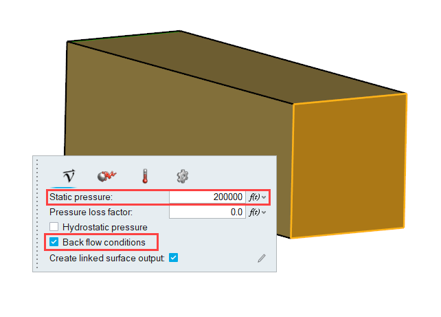
Figure 11. -
In the Turbulence and Temperature tabs, set the back flow type to
Exiting Mass Flux Average
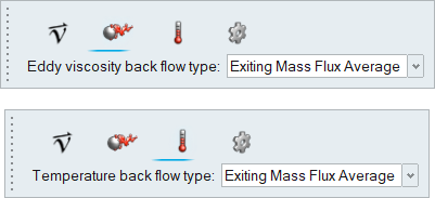
Figure 12. -
On the guide bar, click
to execute
the command and exit the tool.
-
Click the No Slip tool.

Figure 13. -
Select the face highlighted in the figure below then click
 on the guide bar.
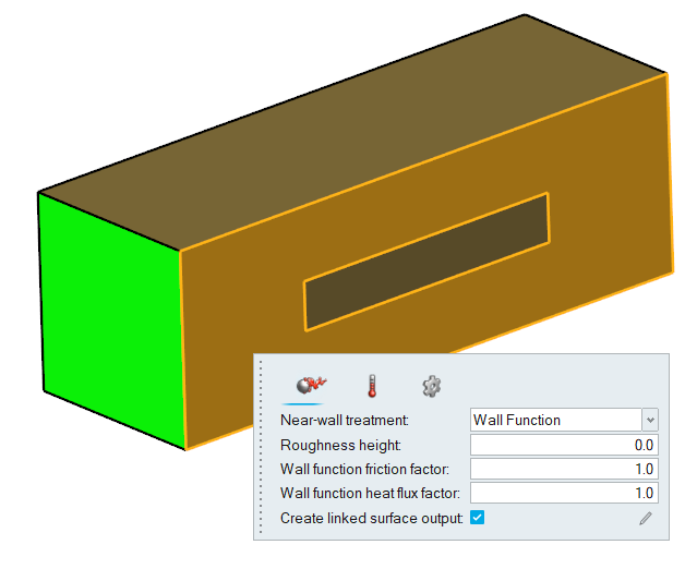
Figure 14. -
In the microdialog, click the
Temperature tab, set the Thermal boundary condition
to Temperature and set the temperature value to
403.15.
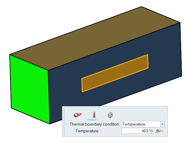
Figure 15. -
Click on the guide bar.
-
Double-click on Wall and rename it to
Bottom.
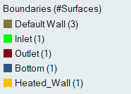
Figure 16. -
Click
 on the guide bar.
Generate the Mesh
-
From the Mesh ribbon, click the
Volume tool.

Figure 17. -
In the Meshing Operations dialog, check that the Mesh
growth rate is set to 1.3.
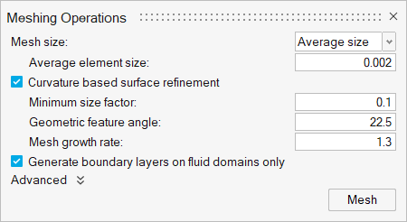
Figure 18.
Run AcuSolve
-
From the Solution ribbon, click the Run tool.

Figure 19.The Launch AcuSolve dialog opens. -
Expand Default initial conditions and enter the values
as shown below to define the initial conditions.
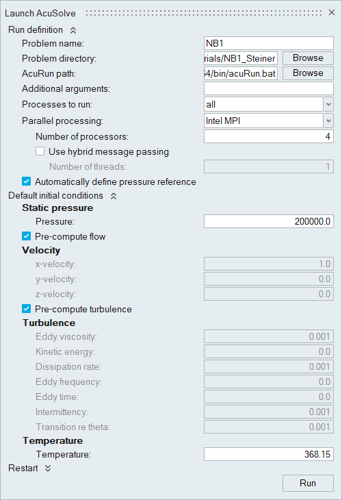
Figure 20.
Post-Process the Results with HW-CFD Post
-
From the Home tools, Files tool group, click the Open Model tool.
Figure 21. -
Select the AcuSolve log file in your problem
directory to load the results for post-processing.
The solid and all the surfaces are loaded in the Post Browser.
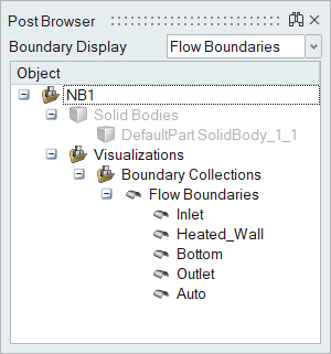
Figure 22. -
Set the Display option to Temperature.
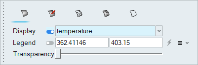
Figure 23. -
Activate the Legend radio button then click
 and set the legend properties as
shown below.
and set the legend properties as
shown below.
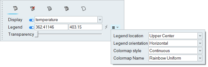
Figure 24.The temperature contours are displayed on the model.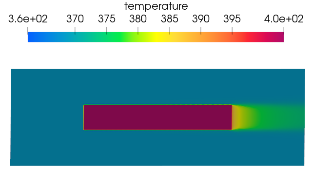
Figure 25.
Summary
In this tutorial, you successfully learned how to set up and solve a simulation involving a single-phase nucleate boiling using HyperWorks CFD. You started by opening the HyperMesh input file with the geometry and then defined the simulation parameters and flow boundary conditions. Once the solution was computed, you used HyperWorks CFD Post to create the contours of temperature.