ACU-T: 3110 Exhaust Manifold Conjugate Heat Transfer - CFD Data Mapping using acuOptiStruct
Prerequisites
This tutorial introduces you to setting up and solving a steady state conjugate heat transfer problem using HyperMesh and then using acuOptiStruct to generate an OptiStruct solver deck to perform a thermal stress analysis. Prior to starting this tutorial, you should have already run through the introductory HyperWorks tutorial, ACU-T: 1000 HyperWorks UI Introduction, and have a basic understanding of HyperMesh, AcuSolve, and HyperView. To run this simulation, you will need access to a licensed version of HyperMesh and AcuSolve.
Prior to running through this tutorial, copy HyperMesh_tutorial_inputs.zip from <Altair_installation_directory>\hwcfdsolvers\acusolve\win64\model_files\tutorials\AcuSolve to a local directory. Extract ACU-T3110_acuOptiStruct.hm from HyperMesh_tutorial_inputs.zip.
Since the HyperMesh database (.hm file) contains meshed geometry, this tutorial does not include steps related to geometry import and mesh generation.
Problem Description

Figure 1. Schematic of Exhaust Manifold
The diameter of the inlets is 0.036 m; the inlet velocity (v) is 8.0 m/s; and the temperature (T) of the fluid entering the inlets is 700 K. The diameter of the outlet is 0.036 m. The pipe wall has a thickness of 0.003 m and the flanges have a thickness of 0.01 m.
The combustion mixture enters the inlets and heat is transferred through conduction inside the manifold. The heat transfer causes deformations and stress in the manifold body which can be simulated using OptiStruct.
- Density (ρ)
- 1.225 kg/m3
- Viscosity (μ)
- 1.781 * 10-5 kg/m-s
- Specific Heat (Cp)
- 1005 J/kg-K
- Conductivity (k)
- 0.0251 W/m-K
- Density (ρ)
- 800 kg/m3
- Specific Heat (Cp)
- 500 J/kg-K
- Conductivity (k)
- 16.2 W/m-K
For the AcuSolve simulation, the variation in material properties of air with temperature is ignored.
The AcuSolve simulation will be set up to model steady state heat transfer to determine the temperature and pressure distribution on the walls of the manifold.
The nodal surface output needs to be activated for all the surfaces in order to create the OptiStruct input deck from the acuOptiStruct command.
The temperature distribution and forces on the wetted surfaces are used by OptiStruct to calculate the deformations and stress in the solid body.
- -solids
- Input name for the solid body/bodies where conduction heat transfer would take place.
- -den
- Density values for the solid body/bodies.
- -spcsurfs
- List of surfaces where boundary condition constraints need to be specified.
- -spcsurfsdof
- List of degrees of freedom for the surfaces.
- -spcsurfsdofvals
- List of degrees of freedom values for the surfaces which is zero by default.
- -type
- Stress analysis type for the OptiStruct solver.
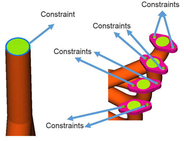
Figure 2.
The stress analysis type is selected as steady linear where the deformations are in the elastic range; that is, the stresses, σ, are assumed to be linear functions of the strains, ε, Hooke's law can be used to calculate the stresses.
Open the HyperMesh Model Database
-
Click the Open Model icon
 located on the standard toolbar.
The Open Model dialog opens.
located on the standard toolbar.
The Open Model dialog opens.
Set the General Simulation Parameters
-
Set the Turbulence model to Spalart Allmaras.
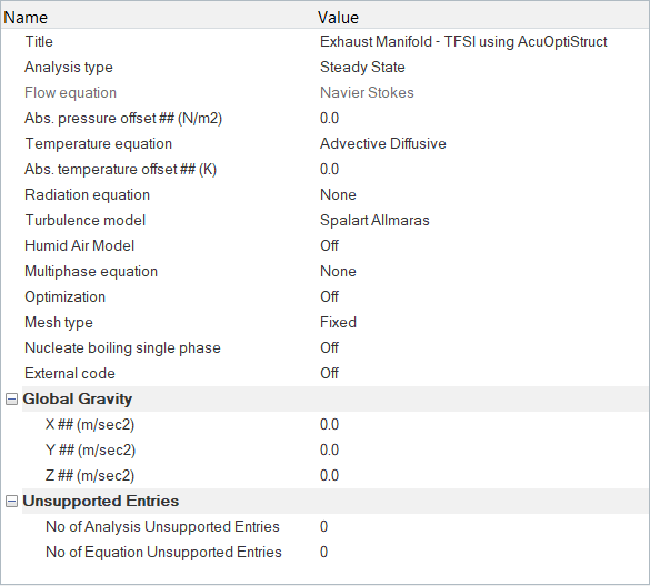
Figure 3.
Assign Material Properties and Boundary Conditions
Create a New Material Model
-
Set the Conductivity to 16.2 W/m-k.
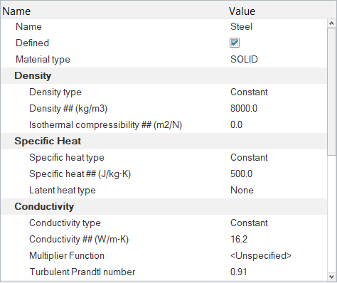
Figure 4.
Assign Material Properties and Boundary Conditions
-
Click Fluid. In the Entity Editor,
- Change the Type to FLUID.
- Set the Material to Air_HM.
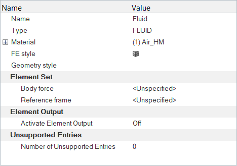
Figure 5. -
Click Solid. In the Entity Editor,
- Change the Type to SOLID.
- Set the Material to Steel.
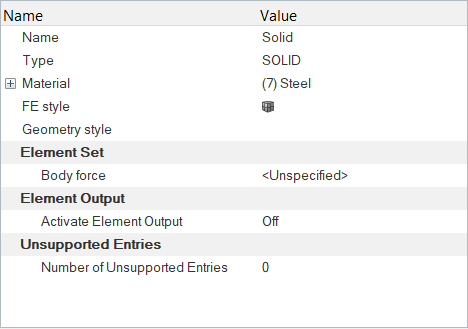
Figure 6. -
Click Inlets. In the Entity Editor,
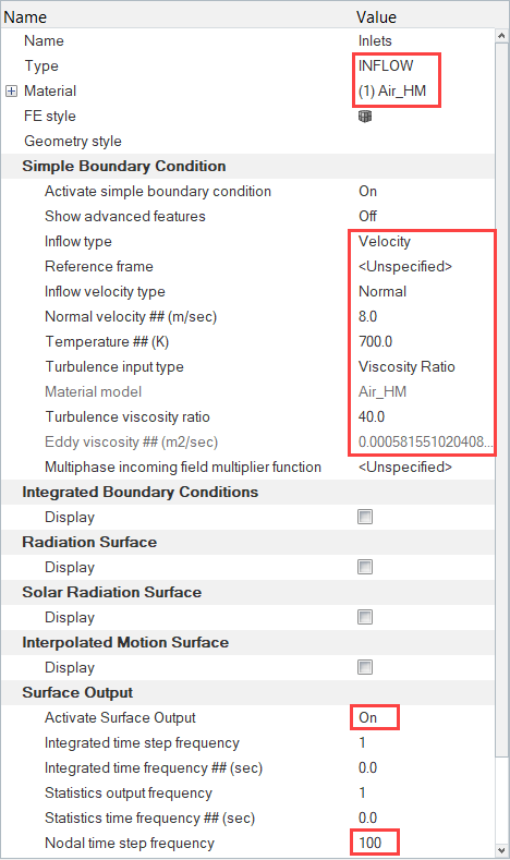
Figure 7. -
Click Outlet. In the Entity Editor,
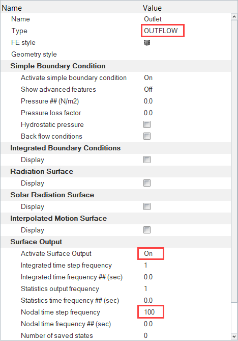
Figure 8. -
Click Outlet_End. In the Entity Editor,
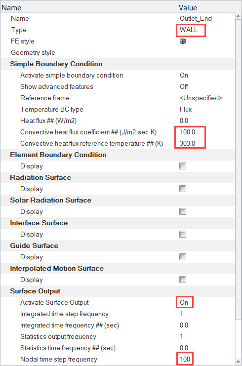
Figure 9. -
Click Outer_Wall. In the Entity Editor,

Figure 10. -
Click Inner_Wall_Fluid. In the Entity Editor,
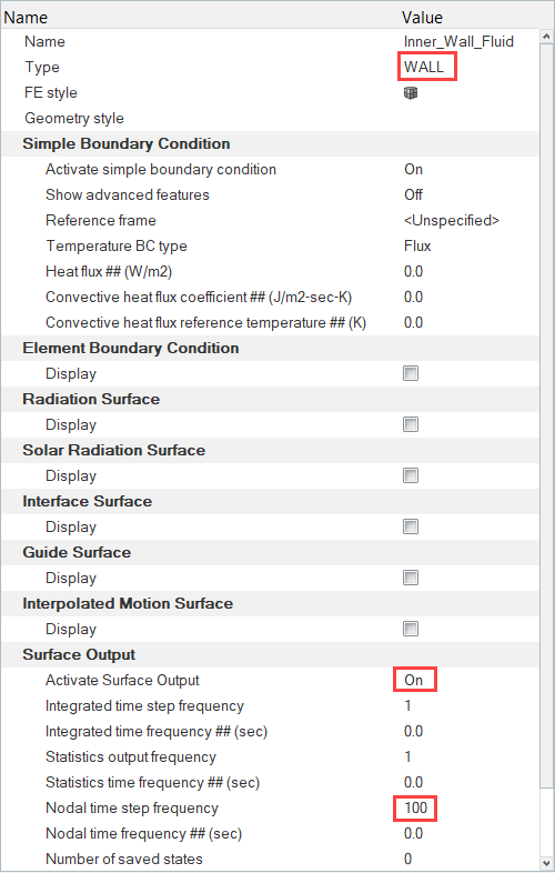
Figure 11. -
Click Inner_Wall_Solid. In the Entity Editor,
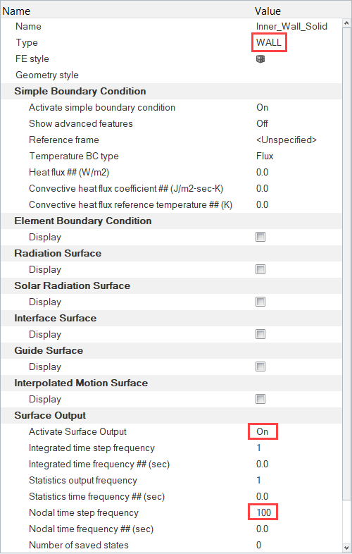
Figure 12. -
Click Flange. In the Entity Editor,
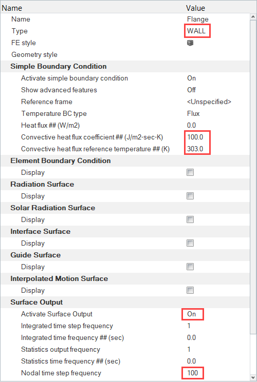
Figure 13. -
Click Flange_Bolts. In the Entity Editor,
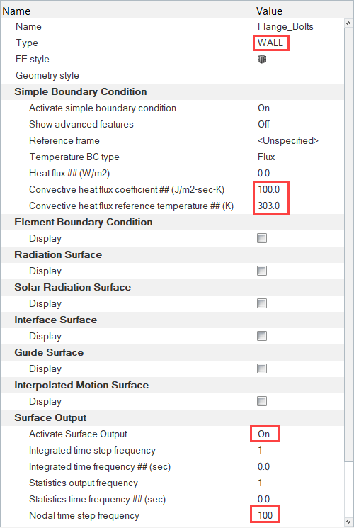
Figure 14. -
In the Solver Browser, click the
Inner_Wall_Fluid component. In the Entity Editor. activate the Interface Surface
Display option and turn On the
interface surface.
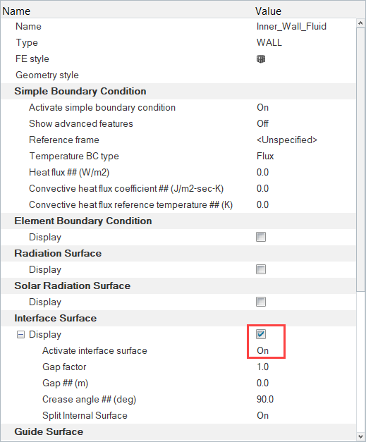
Figure 15. -
Similarly, click the Inner_Wall_Solid component,
activate the Interface Surface Display option, and turn
On the interface surface.

Figure 16.
Define the Nodal Output Frequency
Compute the Solution
-
Click
 on the ACU toolbar.
The Solver job Launcher dialog opens.
on the ACU toolbar.
The Solver job Launcher dialog opens. -
Leave the remaining options as
default and click Launch to start the solution
process.
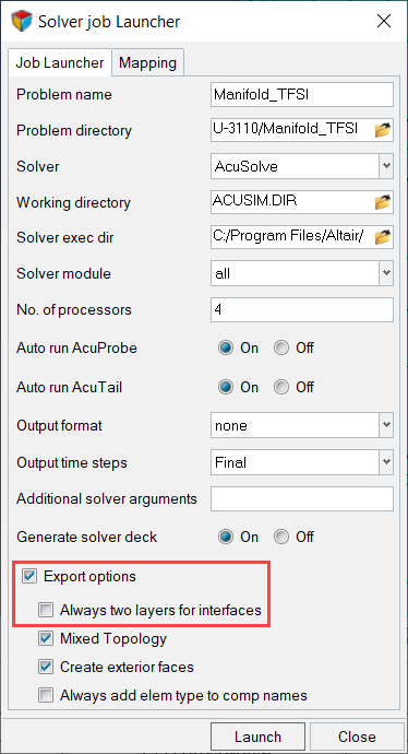
Figure 17.Once you hit the Launch button, the AcuTail and AcuProbe windows are launched automatically. A summary of the run in the AcuTail window indicates that the solver run is complete. Once the run is compete, you can close the AcuTail and AcuProbe windows.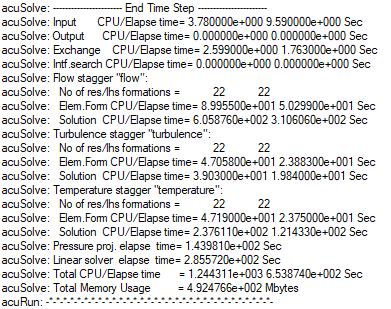
Figure 18.
Use acuOptiStruct to Generate the OptiStruct Solver Deck
Now that the AcuSolve solution has been calculated, you are ready to use the utility ‘acuOptiStruct’ to generate the OptiStruct input deck and run the case using HyperWorks Solver Run Manager. HyperWorks Solver Run Manager is a simple utility which allows to launch any HW solver by selecting appropriate input file(s) and typing any options (if needed) in the field displayed. OptiStruct is an industry proven, modern structural analysis solver for linear and nonlinear structural problems under static and dynamic loadings. OptiStruct can be started directly from the Start menu.
acuOptiStruct uses the flow and thermal data from an AcuSolve conjugate heat transfer CFD simulation to specify the temperature and pressure loads and generates the files necessary to perform a thermal stress analysis using OptiStruct. Executed after the completion of the AcuSolve simulation, acuOptiStruct writes out the solid element mesh data from the AcuSolve run as well as the convective heat transfer information on the wetted surfaces of the solid mesh. Data is written directly in OptiStruct format, both eliminating data loss due to projecting results from one mesh to another and adding fidelity with spatial variation of temperatures and heat transfer coefficients.
In the next steps, you will execute the acuOptiStruct command with the necessary options, which will generate a .fem file. Then you will use OptiStruct to solve the structural problem.
-
Execute the following command:
acuOptiStruct -solids Solids -spcsurfs Flange_Bolts,Outlet_End -spcsurfsdof 123456,123456 -spcsurfsdofvals 0,0 -type sl
This command will generate an OptiStruct input deck from the temperature filed of the flow solution by using the specified constraint surfaces and their degrees of freedom. The analysis type is set to steady linear.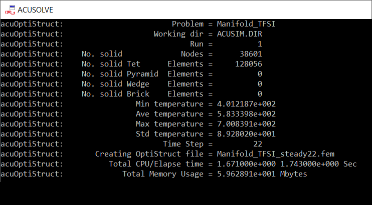
Figure 19. -
Click the
 next to Input
File(s).
next to Input
File(s).
-
Select the .fem file.
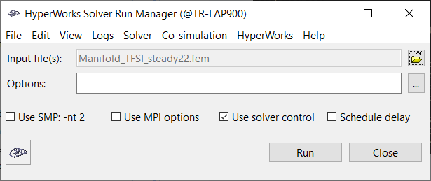
Figure 20. -
Click Run to run the case.
Once the run is complete, the HyperWorks Solver View will show “OptiStruct Job Completed” in the Run summary window.
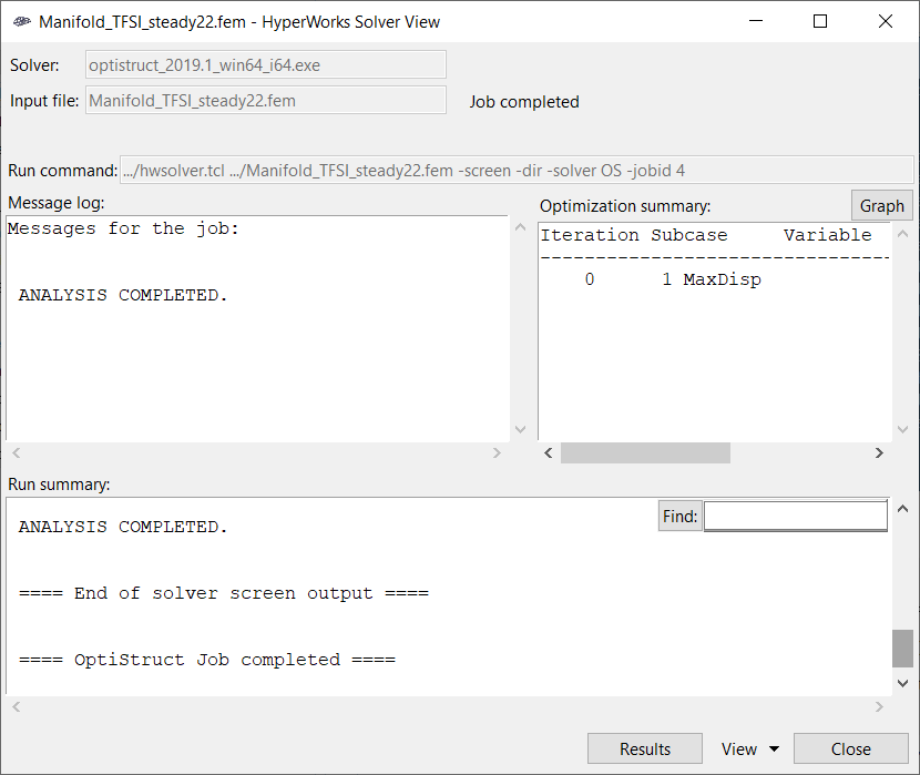
Figure 21.
Post-Process the Results with HyperView
Once the OptiStruct run is complete, close the HyperWorks Solver View dialog. In the HyperMesh Desktop window, close the AcuSolve Control and Solver job Launcher dialogs. In the next few steps, you will plot the contour plot of temperature and pressure on the fluid domain and the displacement and stress contours on the solid domain.
Switch to the HyperView Interface and Load the AcuSolve Model and Results
-
In the HyperMesh Desktop window, click the
ClientSelector drop-down in the bottom-left corner of
the graphics window.
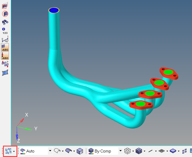
Figure 22. -
In the Load model and results panel, click
 next
to Load model.
next
to Load model.
Create a Contour Plot of Temperature and Pressure
-
Click
 on the Results toolbar to open the Contour panel.
-
In the panel area, click Apply
to plot the temperature contours.
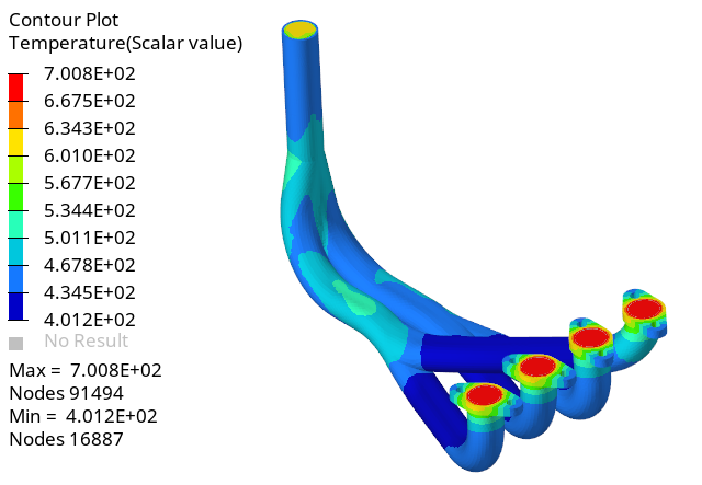
Figure 23. -
Click the Isolate Shown icon
 then click the Inner_Wall_Fluid
component to turn off the display of all components in the graphics window
except the Inner Wall component.
then click the Inner_Wall_Fluid
component to turn off the display of all components in the graphics window
except the Inner Wall component.
-
Click Apply to plot the pressure contours.
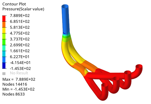
Figure 24.
Load the OptiStruct Results
-
Click on the drop-down beside the Page Window Layout icon
 on
the PageControls toolbar.
on
the PageControls toolbar.
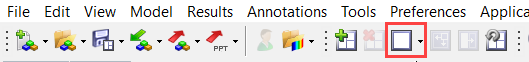
Figure 25. -
In the drop-down menu, select the vertical 2-window layout icon.
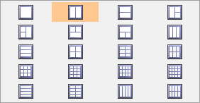
Figure 26. -
Click in the newly created graphics window then click the Load
Results
 icon.
icon.
-
In the Load model and results panel, click next
to Load model.
Create a Contour Plot of Displacement and Element Stresses
-
Click
on the Results toolbar to open the Contour panel.
-
Click Apply to plot the displacement magnitude
contours.
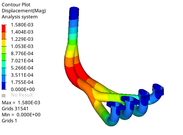
Figure 27. -
Click Apply.
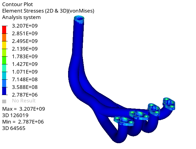
Figure 28.
Summary
In this tutorial you learned how to set up a conjugate heat transfer problem using HyperMesh and solve it using AcuSolve. Once you computed the solution, you used acuOptiStruct to generate the input deck for OptiStruct. Once the solution for the structural analysis was computed, you post-processed the results using HyperView and created contour plots of Temperature, Pressure, Displacement and Stress.