ACU-T: 2200 Transition Flow over an Airfoil using the SST Transition Models
This tutorial provides the instructions for setting up, solving and viewing results for a steady simulation of transition flow over a S809 airfoil using the SST (Shear Stress Transport k-ω) turbulence model with transition models (Gamma or Gamma-ReTheta). AcuSolve is used to compute the intermittency and predict the point where the boundary layer transitions from the laminar mode to turbulence mode. This tutorial is designed to introduce you to the modeling concepts necessary to perform simulations using the transition models coupled with the SST Turbulence model.
- Use of the SST turbulence model with the Gamma transition model
- Use of the SST turbulence model with Gamma-ReTheta transition model
- Analyze the problem
- Start AcuConsole and create a simulation database
- Set general problem parameters
- Set solution strategy parameters
- Import the geometry for the simulation
- Create a volume group and apply volume parameters
- Create surface groups and apply volume parameters
- Set global and local meshing parameters
- Generate the mesh
- Run AcuSolve
- Monitor the solution with AcuProbe
- Post-processing the nodal output with AcuFieldView
Prerequisites
You should have already run through the introductory tutorials, ACU-T: 2000 Turbulent Flow in a Mixing Elbow and ACU-T: 2100 Turbulent Flow Over an Airfoil Using the SST Turbulence Model. It is assumed that you have some familiarity with AcuConsole, AcuSolve, and AcuFieldView. You will also need access to a licensed version of AcuSolve.
Prior to running through this tutorial, copy AcuConsole_tutorial_inputs.zip from <Altair_installation_directory>\hwcfdsolvers\acusolve\win64\model_files\tutorials\AcuSolve to a local directory. Extract s809_blunt.x_t from AcuConsole_tutorial_inputs.zip.
The color of objects shown in the modeling window in this tutorial and those displayed on your screen may differ. The default color scheme in AcuConsole is "random," in which colors are randomly assigned to groups as they are created. In addition, this tutorial was developed on Windows. If you are running this tutorial on a different operating system, you may notice a slight difference between the images displayed on your screen and the images shown in the tutorial.
Analyze the Problem
An important step in any CFD simulation is to examine the engineering problem and determine the important parameters that need to be provided to AcuSolve. Parameters can be based on geometrical components (such as volumes, inlets, outlets, or walls) and on flow conditions (such as fluid properties, velocity, or whether the flow should be modeled as turbulent or as laminar).

Figure 1. S809 Airfoil in the Flow Domain
The diameter of the cylindrical bounding volume for the airfoil is set to 500 times the airfoil chord. This large bounding volume is selected to ensure that the farfield boundaries are sufficiently far from the airfoil to prevent any influence of blockage of the domain on the solution.
The simulation will be carried out by activating the turbulence transition models. The underlying turbulence model used will be the two-equation SST turbulence model. The problem will be solved with the transition models available in AcuSolve – the one-equation Gamma and the two-equation Gamma-ReTheta transition models. As the name suggests, the transition models predict the point where the boundary layer transitions from the laminar mode to turbulence mode. When in the turbulence regime, the SST turbulence model will be used to determine the flow characteristics.
Introduction to Theory
Transition and Transition Models
In the real world, laminar flow and turbulent flow coexist when obstacles are located inside of a fluid flow. Transition flows from laminar to turbulent flow regimes can be found in many industrial applications including turbomachinery, vehicles, drones, and wind turbines.
- Natural Transition: In the laminar flow regime, viscous forces usually damp out the disturbances. However, when the free stream turbulence is low (below 1 percent) and the Reynolds number is higher than the critical Reynolds number, viscous forces destabilize the shear layer, causing the fluid to transition to a turbulent regime via the development of the three initial disturbances (waves, vorticity and vortex breakdown). This mechanism is called the Natural Transition. It is usually very subtle and progresses very slowly, over a long distance scale.
- Bypass Transition: When the initial disturbances are high (due to surface roughness or freestream turbulence levels higher than 1%), turbulence are generated without development of the three initial disturbances (T-S waves, spanwise vorticity, and vortex breakdown) observed in the natural transition.
- Separated-Inducted Transition: When a laminar flow experiences adverse pressure gradients (such as airfoil suction surfaces and flow over a sphere), the fluid flow detaches from the wall surface. If the disturbances are low, separation can cause the generation of structures found in natural transition. Larger disturbances generate Kelvin-Helmholtz instabilities, where vortices roll up before breaking down into turbulence. The process involved in separation-induced transition depends on the size of the adverse pressure gradient and the presence of additional disturbances (for example, obstacles).
Transition Models in AcuSolve
- Gamma-ReTheta Transition Model: The Gamma-ReTheta () model is a correlation-based intermittency model that predicts natural, bypass, and separation-induced transition mechanisms. It is based on two transport equations for intermittency () and transition momentum thickness Reynolds number (). The intermittency is a measure of the flow regime that varies between zero (laminar) and one (fully turbulent). It is used to turn on the turbulent kinetic energy production in the turbulent kinetic energy equation, while the transition momentum thickness Reynolds number is used as the transition onset criteria. The Gamma-ReTheta model is more suitable for cases when freestream turbulence intensity may be high or adverse pressure gradients are present in the flow. Most internal flows and some external flows fall in this category.
- Gamma Transition Model: The Gamma () transition model is a one-equation transition model and follows Galilean invariance by modifying the correlations. The Gamma transition model is well suited for the external aerodynamic cases where freestream turbulence intensity is low.
Transition Model Usage Guidelines
- Meshing Guidelines
- Generate boundary layer meshes on surfaces where transition onset occurs
- The first layer height of the boundary layer mesh should be y+ < 5
- The stretch ratio of the boundary layer mesh should be in the range between 1.1 and 1.2
- The transition between the boundary layer mesh and the freestream mesh should be smooth
- The streamwise surface mesh spacing should be small enough to capture separation bubbles
- Convergence Monitoring
- The residual and solution ratios of the transition simulations are sometimes stagnated (commonly seen when the bubble forms near the leading-edge of an airfoil)
- Despite the appearance of residual and/or solution ratio stagnations, the integrated force and moment over the airfoil could be converged to the satisfactory level. Thus, the monitoring of quantities such as lift, drag, thrust, power, torque, etc. is highly suggested.
The purpose of this tutorial is to provide the instructions for setting up the steady transition simulation of the S809 airfoil using the SST transition models. To keep the total computing time within 5 minutes, some of the meshing guidelines described above have not been followed. However, you must follow these guidelines when solving a problem if a high accuracy in results is desired.
This tutorial consists of two parts. In the first part, you will setup and solve the problem, using the Gamma transition model. After successfully having run the problem with the Gamma model, you will modify the database setup to use the Gamma-ReTheta transition model, and generate the solution again.
Define the Simulation Parameters
Start AcuConsole and Create the Simulation Database
In this tutorial, you will begin by creating a database, populating the geometry-independent settings, loading the geometry, creating volume and surface groups, setting group attributes, adding geometry components to groups and assigning mesh controls and boundary conditions to the groups. Next you will generate a mesh and run AcuSolve to solve for the number of time steps specified. Finally, you will review some characteristics using AcuFieldView.
In the next steps you will start AcuConsole and create the database for storage of the simulation settings.
-
Click the File menu, then click
New to open the New data
base dialog.
Note: You can also open the New data base dialog by clicking
 on the toolbar.
Define Expressions and Variables Using the Variable Manager
In this step, you will use the Variable Manager in AcuConsole to create a list of expressions that will be used during the model setup process.
-
Click the Variable List icon from the main
toolbar:

Figure 2.The Variable Manager opens.
-
Repeat this process for the remaining variables shown in the table below:
Name Expression Description Uinf 4.0 Free Stream Velocity of Air alpha 1.0 Angle of attack (degrees) xVelocity :=Uinf * cos(alpha*deg) X component of velocity yVelocity :=Uinf * sin(alpha*deg) Y component of velocity Once the expressions are entered, the Variable Manager should appear similar to what is shown below: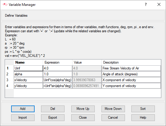
Figure 3.
Set General Simulation Parameters
In next steps you will set parameters that apply globally to the simulation. To make this simple, the basic settings applicable for any simulation can be filtered using the BAS filter in the Data Tree Manager. This filter enables display of only a small subset of the available items in the data tree and makes navigation of the entries easier.
-
Click BAS in the Data Tree Manager to switch to basic view in the Data Tree.
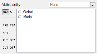
Figure 4. -
Change the Turbulence transition model from None to
Gamma.
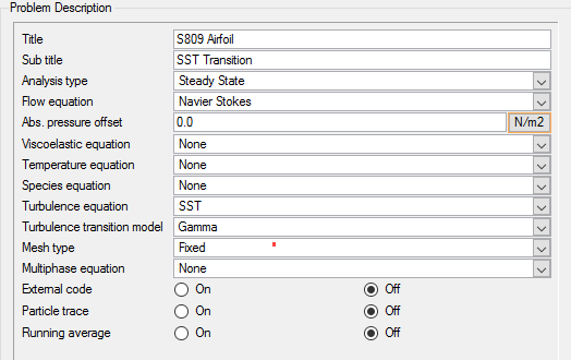
Figure 5.
Set Solution Strategy Parameters
-
Ensure that both the Turbulence and Turbulence transition flags are set to
On.
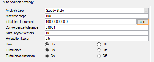
Figure 6.
Set Material Model Parameters
AcuConsole has three pre-defined standard materials, Air, Aluminium, and Water, with standard parameters defined. In the next steps you will check and if needed modify the material characteristics of the predefined "Air" model to match the desired properties for this problem.
-
Double-click Material Model
in the Data Tree to expand it.
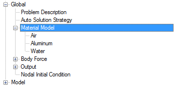
Figure 7.
The remaining thermal and other material properties are not critical to this simulation. However, you may browse through the tabs to check the complete material specification.
-
Save the database to create a backup
of your settings. This can be achieved with any of the following
methods.
- Click the File menu, then click Save.
- Click
 on
the toolbar.
on
the toolbar. - Click Ctrl+S.
Note: Changes made in AcuConsole are saved into the database file (.acs) as they are made. A save operation copies the database to a backup file, which can be used to reload the database from that saved state in the event that you do not want to commit future changes.
Import the Geometry and Define the Model
Import Airfoil Geometry
-
Select s809_blunt.x_t and click
Open to open the Import Geometry
dialog.
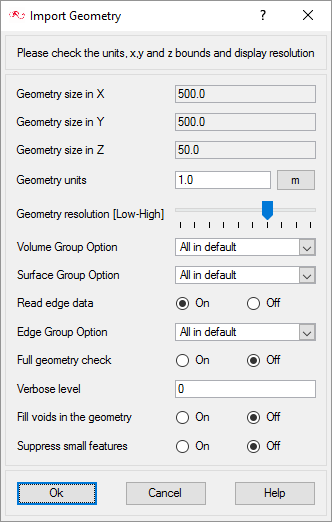
Figure 8.For this tutorial, the default values for the Import Geometry dialog are used to load the geometry. If you have previously used AcuConsole, be sure that any settings that you might have altered are manually changed to match the default values shown in the figure. With the default settings, volumes from the CAD model are added to a default volume group. Surfaces from the CAD model are added to a default surface group. You will work with groups later in this tutorial to create new groups, set flow parameters, add geometric components, and set meshing parameters.
-
Rotate and zoom in the visualization to view the entire model.

Figure 9.
Apply Volume Parameters
Volume groups are containers used for storing information about a volume region. This information includes solution and meshing parameters applied to the volume and the geometric regions that these settings are applied to.
When a new geometry is imported, by default AcuConsole will place all volumes from a geometry in a single volume container named "default". You should be able to see it in the data tree upon successful import of your model in the last step, under .
Since the model for this tutorial has only a single volume, it will be the only volume in the default volume group when the geometry is imported. Even when there is a single volume in the model, it is advisable to rename the volume for ease of identification in future. In the next steps you will rename the default volume group container, and set the material and other properties for it.
-
Minimize Global in the Data Tree Manager and expand the Model
tree item by clicking
 .
.
-
Toggle the display of the default volume container by clicking
 and
and
 next to the volume name.
Note: You may not see any change when toggling the display if Surfaces are being displayed, as surfaces and volumes may overlap.
next to the volume name.
Note: You may not see any change when toggling the display if Surfaces are being displayed, as surfaces and volumes may overlap. -
Set up the fluid volume element set.
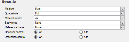
Figure 10.
Create Surface Groups
Surface groups are containers used for storing information about a surface, including solution and meshing parameters, and the corresponding surface in the geometry that the parameters will apply to.
In the next steps you will define surface groups, assign the appropriate attributes for each group in the problem and add surfaces to the groups.
In the process of setting up a simulation, you need to move into different panels for setting up the boundary conditions, mesh parameters, etc. which can sometimes be cumbersome (especially for models with too many surfaces). To make it easier, less error prone, and for saving time two new dialogs are provided in AcuConsole which you can use to verify and provide the information for all surface or volume entities at once. They are the Volume Manager and Surface Manager. In this section some features of Surface Manager are exploited.
-
Rename Surface Names (column 1) for Surface 1 to Surface 3, and set the Simple
BC Active and Simple BC Type columns as per the table shown below.
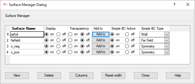
Figure 11. -
Assign the surfaces to the z_pos and z_neg surface groups.
-
Similarly assign the surface with the minimum z-coordinate to the z_neg
surface group.
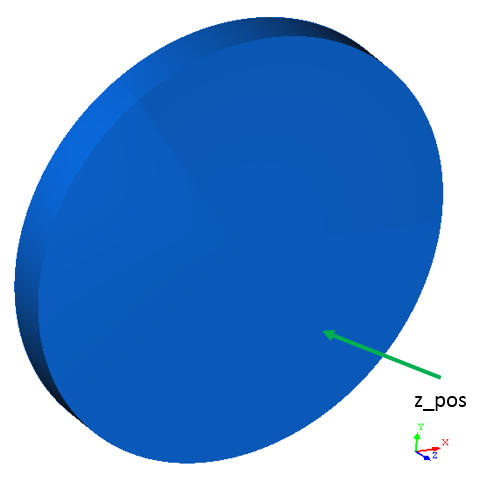
Figure 12.
-
Similarly assign the surface with the minimum z-coordinate to the z_neg
surface group.
-
Assign the outer peripheral surface of the domain to the farfield surface
group. Use the following figure as the reference for selecting the required
surfaces.
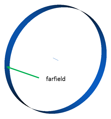
Figure 13.When the geometry was loaded into AcuConsole, all geometry surfaces were placed in the default surface group container. This default surface group was renamed to airfoil. In the previous steps, you assigned some surfaces to various other surface groups that you created. At this point, all that is left in the airfoil surface group are the surfaces which make up the airfoil.
Assign the Surface Parameters
-
Set up the farfield surface parameters:
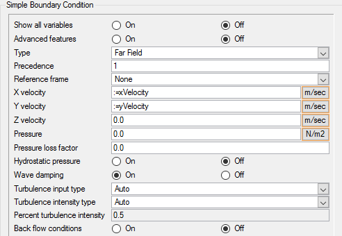
Figure 14.You can see the value of Percent turbulence intensity is set to 0.5. This value is automatically selected by AcuConsole based on parameters like the turbulence model selected, flow type, etc.
Set Initial Conditions
For the SST turbulence model, you need to provide the initial value for kinetic energy and eddy frequency. For the Gamma transition model, you need to provide the initial value for Intermittency, or . If you have a reasonable estimate of these values, you can enter them directly in the nodal initial condition fields. One option is to use the same values that are assigned at the inlet boundary. In the absence of good estimates for the initial conditions, it is also possible to let AcuSolve perform an automatic initialization of the turbulence and transition variables. By setting these values to zero, AcuSolve will trigger an automatic initialization of these variables.
-
Set the Kinetic energy, Eddy frequency and Intermittency to
0.0 to trigger the automatic initialization.
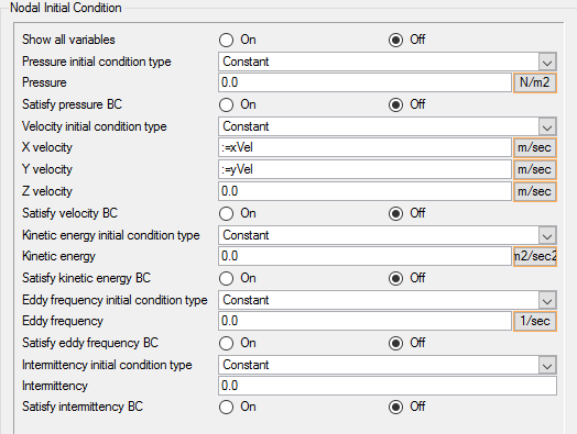
Figure 15.
Assign Mesh Controls
Set Global Meshing Parameters
Now that the flow characteristics have been set for the whole problem, a sufficiently refined mesh has to be generated.
Global mesh attributes are the meshing parameters applied to the model as a whole without reference to a specific geometric volume, surface, edge, or point. Local mesh attributes are used to create mesh generation controls for specific geometry components of the model.
In the next steps you will set the global mesh attributes.
-
Set Maximum sweep angle to 5.0 degrees.
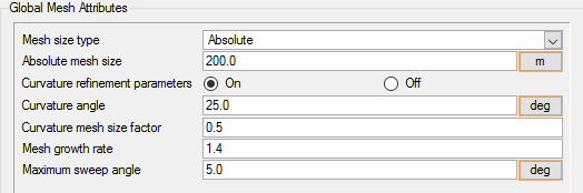
Figure 16.
Set Mesh Process Parameters
For this simulation, the mesher will locally reduce the height of the boundary layer stack but will keep the total number of layers constant. Using this approach, the height of each layer is scaled by a constant factor to reduce the total height of the stack and avoid the creation of the poor quality boundary layer elements.
-
Set the 2D Boundary layer adjacent height smoothing ratio to
0.25.
This parameter controls how smoothly the local boundary layer heights vary from one element to the next after the layers height are adjusted locally to resolve poor quality elements. A low value of this parameter smooths the variation in height over a large distance, while a value closer to 1.0 enforces a more abrupt change in height. Note that there are separate values of this setting for 2D and 3D boundary layers. For this application, you will be creating a 2D mesh and extruding it in the third direction to create the volume. Therefore, the 2D setting will control the behavior of the mesh in this case.
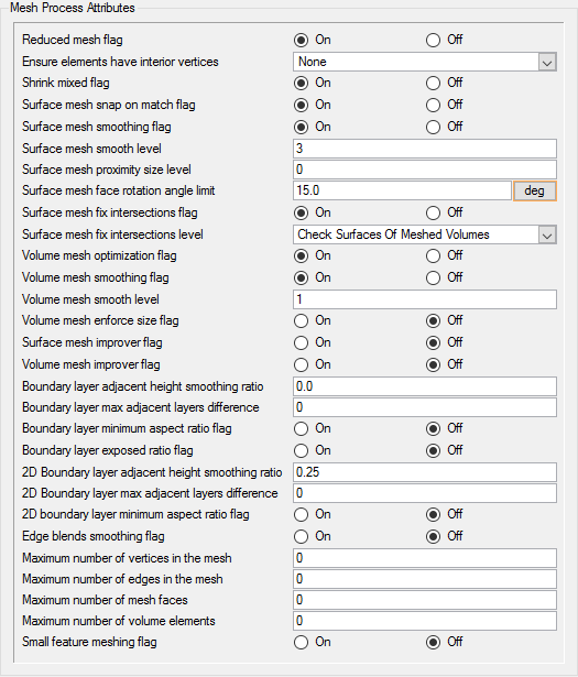
Figure 17.
Set Surface Mesh Parameters
Surface mesh attributes are applied to a specific surface in the model. It is a type of local meshing parameter used to create targeted mesh controls for one or more specific surfaces.
Setting local mesh attributes, such as surface mesh attributes, is not mandatory. When a local mesh attribute is not found for a component, the global attributes are used as the mesh generation control for that component. If a local mesh attribute is present, it will take precedence over the global setting.
In the next steps you will set the surface meshing attributes.
-
Set the remaining parameters as follows:
- First element height: 0.0004
- Total layer height: 0.04
- Growth rate: 1.2
- Boundary layer elements type: Tetrahedron
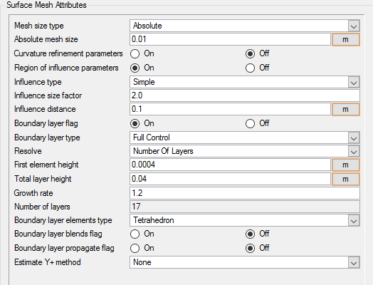
Figure 18.
Set Edge Mesh Parameters
To create an optimum mesh on the surface of the airfoil, it is necessary to have high levels of refinement near the leading and trailing edges and a large element size near the mid chord. Since our surface mesh size was set to constant to serve as the size that is propagated into the volume for the region of influence refinement, you will use an edge mesh attribute to control the placement of nodes along the airfoil surface. To accomplish this, you will first need to create an edge group that contains the perimeter edges of the airfoil.
-
Select the two perimeter edges of the airfoil to add them to this group.
-
Click Done.
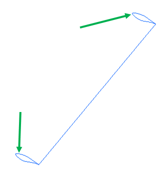
Figure 19.
-
Click Done.
Define Mesh Extrusion
The present simulation is equivalent to a representation of a 2D cross section of the model. In AcuSolve 2D models are simulated by having just one element across the faces of the cross section. Thus when these faces are set up with a similar boundary condition, it coerces the corresponding nodes across the faces to have same results. In this problem, these faces are the negative and positive z-surfaces. This kind of mesh is achieved in AcuSolve with mesh extrusion process. In the following steps you will define the process of extrusion of the mesh between these surfaces.
-
Click OK to accept these settings.
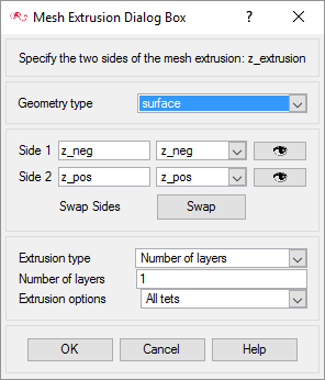
Figure 20.
Generate the Mesh
In the next steps you will generate the mesh that will be used when computing a solution for the problem.
-
Click
 on the toolbar to open the Launch
AcuMeshSim dialog.
on the toolbar to open the Launch
AcuMeshSim dialog.
-
Leave the default settings and select OK.
During meshing an AcuTail window opens. Meshing progress is reported in this window. A summary of the meshing process indicates that the mesh has been generated.
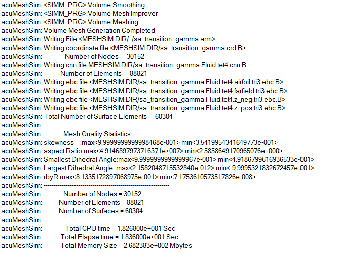
Figure 21.Note: The actual number of nodes and elements, and memory usage may vary slightly from machine to machine. -
You can rotate and zoom in the model to analyse the various mesh regions.
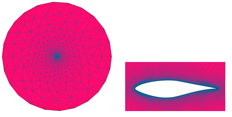
Figure 22.
Compute the Solution and Review the Results
Run AcuSolve
In the next steps, you will launch AcuSolve to compute the solution for this case.
-
Click
 on the toolbar to open the
Launch AcuSolve dialog.
For this case, the default settings will be used. AcuSolve will run using four processors (if available, higher number of processors may be specified) and AcuConsole will generate AcuSolve input files and will launch AcuSolve. AcuSolve will calculate the steady state solution for this problem.
on the toolbar to open the
Launch AcuSolve dialog.
For this case, the default settings will be used. AcuSolve will run using four processors (if available, higher number of processors may be specified) and AcuConsole will generate AcuSolve input files and will launch AcuSolve. AcuSolve will calculate the steady state solution for this problem. -
Select Ok to start the solution process.
While computing the solution, an AcuTail window opens. Solution progress is reported in this window. A summary of the solution process indicates that the run has been completed.
The information provided in the summary is based on the number of processors used by AcuSolve. If you use a different number of processors than indicated in this tutorial, the summary for your run may be slightly different than the summary shown.
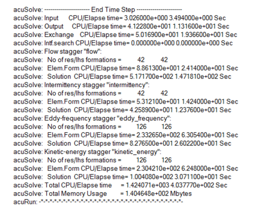
Figure 23.
Post-Process with AcuProbe
AcuProbe can be used to monitor various variables over solution time.
-
Open AcuProbe by clicking
 on the toolbar.
-
Right-click Final and click Plot
All.
This will plot the residuals for all the variables, pressure, velocity, eddy viscosity, and intermittency, in the plot area.Note: You might need to click
 on the toolbar in order to
properly display the plot.
on the toolbar in order to
properly display the plot.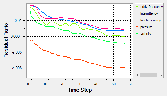
Figure 24. -
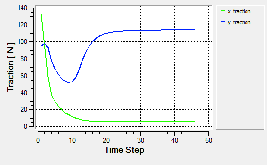
Right-click on x-traction and select
Plot then right-click on
y-traction and select plot
Plot.
Note: You might need to click on the toolbar in order to
properly display the plot.
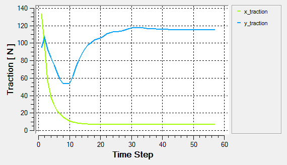
Figure 25.The traction values on the airfoil surface have nearly converged. When using correlation-based transition models, it is always a good practice to examine not only the residuals but also the actual solution quantities of interest for convergence before accepting the solution. In some other cases, it is also possible that the flow field has converged even while the residuals show minor oscillations. The user thus should observe both in tandem before taking an informed decision about the validity of the solution.
Post-Process with AcuFieldView
- How to find the data readers in the File menu and open up the desired reader panel for data input.
- How to find the visualization panels either from the Side toolbar or the Visualization panel menu to create and modify surfaces in AcuFieldView
- How to move the data around the graphics window using mouse actions to translate, rotate and zoom in to the data.
-
Click
 on the
AcuConsole toolbar to open the
Launch AcuFieldView dialog.
on the
AcuConsole toolbar to open the
Launch AcuFieldView dialog.
-
Click OK to start AcuConsole.
You will see that the pressure contours have already been displayed on all the boundary surfaces with mesh.
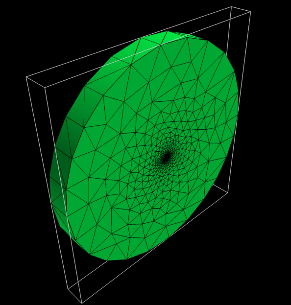
Figure 26.
Set Up AcuFieldView
-
Click Viewer Options.
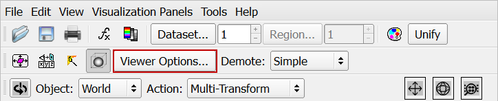
Figure 27. -
On the toolbar, click the Colormap icon
 .
.
-
Click the Toggle Outline icon
 on the toolbar to turn off the outline display.
Your display should look similar to Figure 2.
on the toolbar to turn off the outline display.
Your display should look similar to Figure 2.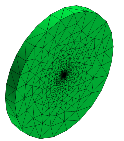
Figure 28.
Coordinate the Surface Showing Turbulence Viscosity on the Mid Coordinate Surface
-
Click
 to open
the Coordinate Surface dialog.
to open
the Coordinate Surface dialog.
-
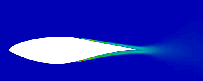
From the Defined Views menu, select +Z as the viewing
direction.
Your view should be similar to Figure 1.
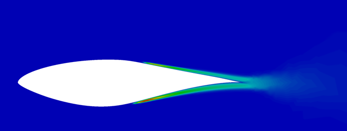
Figure 29.You can clearly see the turbulent flow developing at about halfway through the chord of the airfoil. Before the onset of turbulence, the boundary layer on the airfoil surface is laminar.
-
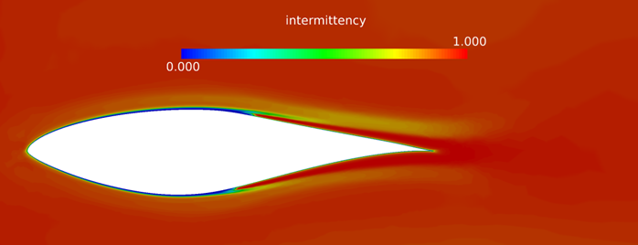
Open the Coordinate Surface dialog, click
Select next to Scalar Function and select
Intermittency.
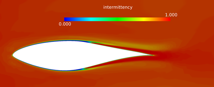
Figure 30.A closer look at the contour plot of intermittency will show that the value of intermittency transitions to one at the point where the flow transitions from laminar to turbulent. In the region where the flow is laminar, from the leading edge of the airfoil to the halfway, the intermittency is zero.
Post-Process to Calculate Flow Coefficients
AcuSolve is shipped with a number of utility scripts to facilitate the pre and post-processing of a problem solved using the solver. You will be introduced to two of these scripts, AcuLiftDrag and AcuGetCpCf in this section, and their usage. These two scripts are focused on aerodynamic simulations as the ones solved in this tutorial.
Run AcuLiftDrag
AcuLiftDrag is a utility script used to calculate the lift and drag coefficients for an airfoil.
In the Analyze the Problem section, it was described that the simulation is performed as 2D by including only a single layer of extruded elements in the airfoil span direction. When solving a problem in such a way, the span of the airfoil should be set equal to the thickness of the domain in the extrusion direction. When solving a 3D problem, the actual span of the airfoil should be used.
To execute the AcuLiftDrag script for this position, follow the steps below:
-
Enter the following command at the prompt:
acuLiftDrag -osis airfoil -aoa 1 -ref_vel 4 -chord 1 -rho 1.225
-span 50
The output of the command should look like the image below: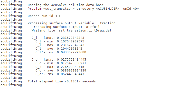
Figure 31.The value C_l corresponds to the lift coefficient, and C_d corresponds to the drag coefficient. The final keyword refers to the respective coefficient values at the last time step of the simulation. The rest of the values provide the basic statistics for these coefficients over all the time steps of the simulation. These statistics are more meaningful if the simulation is transient.
The script also creates the file Turbulent_Airfoil_SST.liftDrag.dat in the problem directory. The file contains the lift and drag data for all the available time steps in a determined tabular arrangement. The first column is the time step, the second column is the lift coefficient, and the third column is the drag coefficient.
Run AcuGetCpCf
AcuGetCpCf is another utility script used to calculate the pressure coefficient (Cp) for the airfoil.
To execute the AcuGetCpCf script for this problem, follow the steps below:
-
Enter the following command at the prompt:
acuGetCpCf -osis airfoil -type cp -ref_vel 4 -rho
1.225 -no_nc
The output of the command should look like the image below:
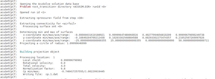
Figure 32.The script prints the minimum and maximum vlaues for the presure coefficient. It also creates a file, cp.1.dat, in the problem directory. The file contains the pressure coefficient data along the chord of the airfoil. The first column is the x-coordinate along the chord, and the second column is the pressure coefficient. You can use an external plotting utility to the plot the data. The resulting plot is shown below.

Figure 33.
Set Up the Gamma-ReTheta Transition Model
At this stage you have successfully setup and ran the S809 airfoil problem with the Gamma transition model and SST turbulence model. In this part of the tutorial you will modify your open database to setup the problem so as to use the Gamma-ReTheta transition model.
- Close the open AcuFieldView window and return to the open AcuConsole window.
- Save the database to retain the setup for the Gamma transition model.
- Create a new directory within your existing working directory, or at any other location of your choice, and name it SST_Gamma_ReTheta.
- Click
- Navigate into the SST_Gamma_Re_Theta directory. Enter sst_transition_gammaretheta as the File name for the database, or choose any name of your preference.
- Save the database to create a backup of your settings.
Update General Simulation Parameters
-
Click BAS in the Data Tree Manager to switch to basic view in the Data Tree.
Figure 34. -
Change the Turbulence transition model from Gamma to
Gamma-ReTheta.
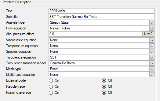
Figure 35.
Update the Nodal Initial Conditions
The Gamma-ReTheta transition model is a two equation model and introduces a new variable, transition ReTheta, or . Like other variables, an initial value for this variable also needs to be provided. As before, you will set it to zero to trigger the automatic initialization of by AcuSolve.
-
Set Transition re theta to 0.0 to trigger the automatic
initialization.
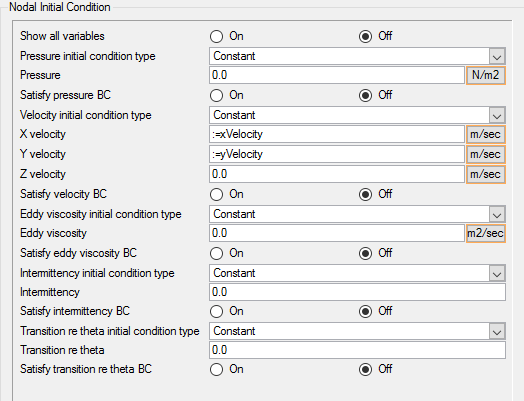
Figure 36.The remaining settings in the setup need not be modified. You can now launch AcuSolve to get the solution of the S809 airfoil problem with the Gamma-ReTheta transition case. Follow the same steps as in the previous case to post-process the results.
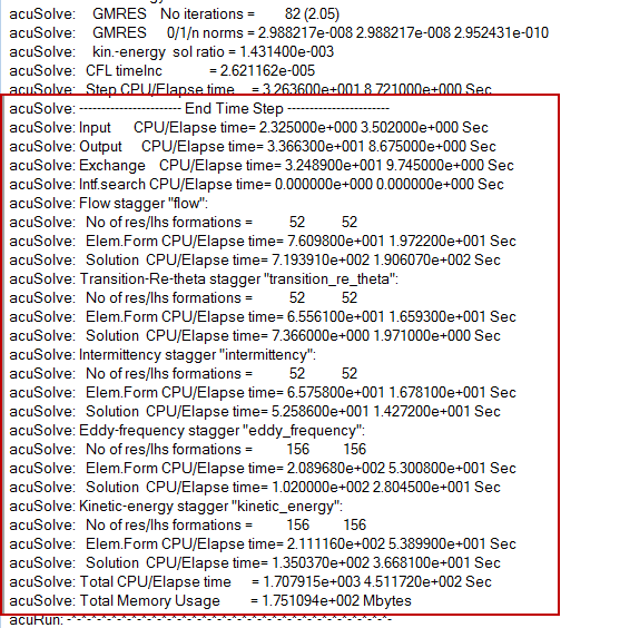
Figure 37.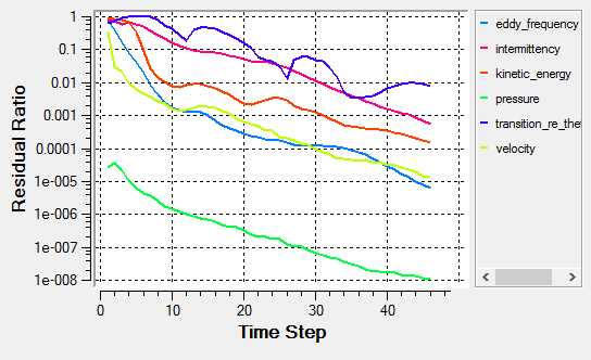
Results from running AcuLiftDrag and AcuGetCpCf on the Gamma-Re Theta database are shown below:
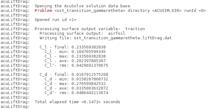
Figure 38.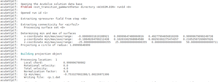
Figure 39.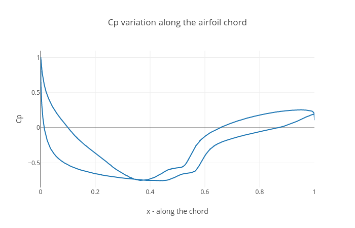
Figure 40.
Summary
In this AcuSolve tutorial, you successfully set up and solved a turbulence transition problem. The underlying turbulence model employed was the SST model. The problem simulated a S809 wind turbine airfoil in an external flow field. You started the tutorial by creating a database in AcuConsole, importing and meshing the geometry, and setting up the simulation parameters. The database was initially set up with the one-equation Gamma transition model. Once the case was setup, the solution was generated with AcuSolve. Results were post-processed in AcuProbe and AcuFieldView. In AcuFieldView you observed the inter-relation between onset of turbulence viscosity and intermittency. After successfully getting a solution for the Gamma transition model, you modified the database to use the two-equation Gamma-ReTheta as the transition model.