ACU-T: 2100 Turbulent Flow Over an Airfoil Using the SST Turbulence Model
This tutorial provides the instructions for setting up and using the SST and K-Omega turbulence models in AcuSolve. The application that is investigated is the flow over a NACA0012 airfoil at an angle of attack of 5 degrees. AcuSolve is used to extract the lift and drag forces on the airfoil. This tutorial is designed to introduce you to the modeling concepts necessary to perform external aerodynamic simulations using the SST and K-Omega turbulence models.
- Use of the SST and/or K-Omega turbulence models
- Use of the farfield boundary condition type
- Use of the Variable Manager to store variables and expressions
- Entry of expressions into the panel area.
Prerequisites
You should have already run through the introductory tutorial, ACU-T: 2000 Turbulent Flow in a Mixing Elbow. It is assumed that you have some familiarity with AcuConsole, AcuSolve, and AcuFieldView. You will also need access to a licensed version of AcuSolve.
Prior to running through this tutorial, copy AcuConsole_tutorial_inputs.zip from <Altair_installation_directory>\hwcfdsolvers\acusolve\win64\model_files\tutorials\AcuSolve to a local directory. Extract NACA0012.x_t from AcuConsole_tutorial_inputs.zip.
Analyze the Problem
An important first step in any CFD simulation is to examine the engineering problem to be analyzed and determine the settings that need to be provided to AcuSolve. Settings can be based on geometrical components (such as volumes, inlets, outlets, or walls) and on flow conditions (such as fluid properties, velocity, or whether the flow should be modeled as turbulent or as laminar).
The problem to be addressed in this tutorial is shown schematically in the figure below. It consists of a cylindrical bounding region containing air that flows past a NACA0012 airfoil profile. The simulation is performed as 2D by including only a single layer of extruded elements in the airfoil span direction. The velocity vector at the far field boundary of the domain is specified to yield an angle of attack of 5 degrees and a Reynolds Number of 1.0e6. The airfoil chord is 1 meter, and standard air material properties are used for the simulation.

Figure 1.
The diameter of the cylindrical bounding volume for the airfoil is set to 500 times the airfoil chord. This large bounding volume is selected to ensure that the farfield boundaries are sufficiently far from the airfoil to prevent any influence of blockage of the domain on the solution.
The initial simulation of this airfoil will be considered fully turbulent and use the SST turbulence model. These simulation conditions correspond to a scenario where the boundary layer on the leading edge of the airfoil is tripped with some type of roughness elements to produce a fully turbulent boundary layer over the length of the airfoil.
Define the Simulation Parameters
Start AcuConsole and Create the Simulation Database
In this tutorial, you will begin by creating a database and loading some predefined variables, populating the geometry-independent settings, loading the geometry, creating groups, setting group attributes, adding geometry components to groups and assigning mesh controls and boundary conditions to the groups. Next you will generate a mesh and run AcuSolve to converge on a steady state solution. Finally, you will review the results using AcuFieldView and AcuProbe.
In the next steps you will start AcuConsole, create the database for storage of AcuConsole settings and set the location for saving mesh and solution information for AcuSolve.
-
Click the File menu, then click
New to open the New data
base dialog.
Note: You can also open the New data base dialog by clicking
 on the toolbar.
Define Expressions and Variables Using the Variable Manager
In this step, you will use the Variable Manager in AcuConsole to create a list of expressions that will be used during the model setup process.
The Variable Manager is a useful utility that allows you to define variables and expressions that can later be referenced as inputs to the various settings used throughout the process of building your model. When a model is constructed in terms of variables, it is very easy to update the entire model with a simple change of a single parameter from the Variable Manager. This process will be illustrated in this tutorial.
| Name | Expression |
|---|---|
| volumeFlowRate | =2*2 |
| Name | Expression |
|---|---|
| inletArea | 2.0 |
| averageVelocity | 2.0 |
| volumeFlowRate | :=inletArea*averageVelocity |
Using this syntax, the formula for volumeFlowRate is stored in the database and will automatically update whenever the inletArea or averageVelocity are updated. Any variables that are defined in the Variable Manager can be referenced when specifying an integer or floating point value in the panels area. The same expression syntax can be used.
-
Click the Variable List icon from the main
toolbar:

Figure 2.The Variable Manager opens.
-
Repeat this process for the remaining variables shown in the table below:
Name Expression Description ReynoldsNumber 1000000 Target Reynolds number for the simulation rho 1.225 Density of air mu 1.781e-5 Molecular viscosity of air chord 1.0 Airfoil chord alpha 5.0 Angle of attack (degrees) windSpeed :=ReynoldsNumber*mu/(rho*chord) Velocity of air (m/s) xVelocity :=windSpeed*cos(alpha*deg) X component of velocity yVelocity :=windSpeed*sin(alpha*deg) Y component of velocity turbIntensityPercent 0.025 Turbulence intensity percentage viscosityRatio 0.03 Viscosity ratio (turbulent viscosity / molecular viscosity) globalMeshSize :=200*chord Global maximum element size surfaceMeshSize :=.02*chord Maximum surface element size firstLayerHeight 1.2e-5 Boundary layer first layer height stretchRatio 1.2 Boundary layer element growth rate totalLayerHeight 0.004 Total height of boundary layer element stack sweepAngle 7.0 Sweep angle for boundary layer blends at sharp edges Once the expressions are entered, the Variable Manager should appear similar to what is shown below: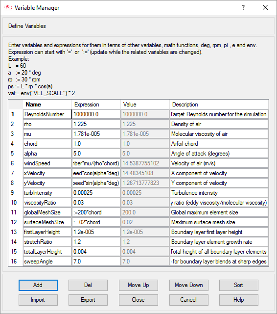
Figure 3.
Set General Simulation Parameters
In the next steps you will set parameters that apply globally to the simulation. To simplify this task, you will use the BAS filter in the Data Tree Manager. The BAS filter limits the options in the Data Tree to show only the basic settings.
The general attributes that you will set for this tutorial are for turbulent flow, and steady state time analysis.
-
Click BAS in the Data Tree Manager to switch to basic view in the Data Tree.
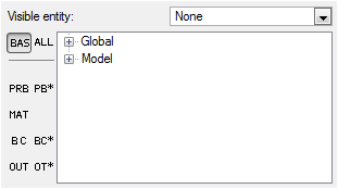
Figure 4. -
Double-click the Global
Data Tree item to expand it.
Tip: You can also expand a tree item by clicking
 next to the item name.
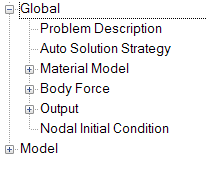
Figure 5. -
Change the Turbulence equation to
SST
The SST and K-Omega models both require the same set of inputs, so the steps in this tutorial also apply to the K-omega model. If you wish to use the K-Omega model instead of SST, you can select it from this menu.
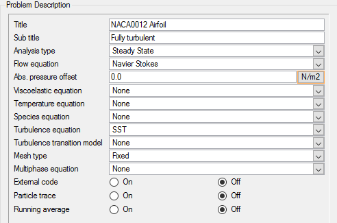
Figure 6.
Set Solution Strategy Parameters
In the next steps you will set the parameters that control the behavior of AcuSolve as it progresses during the transient solution.
-
Enter 0.4 for Relaxation factor.
This value is used to improve convergence of the solution. Typically a value between 0.2 and 0.4 provides a good balance between achieving a smooth progression of the solution and the extra compute time needed to reach convergence. Higher relaxation factors cause AcuSolve to take more time steps to reach a steady state solution. A high relaxation factor is sometimes necessary in order to achieve convergence for very complex applications.
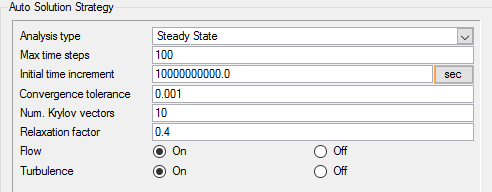
Figure 7.
Set Material Model Parameters
In the next steps you will modify the pre-defined material properties of air using an expression that was created in the Variable Manager.
-
Double-click Material Model
in the Data Tree to expand it.
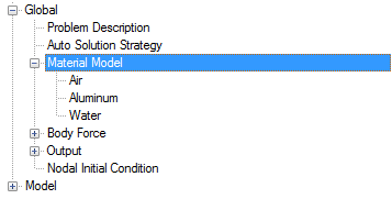
Figure 8. -
Save the database to create a backup
of your settings. This can be achieved with any of the following
methods.
- Click the File menu, then click Save.
- Click
 on
the toolbar.
on
the toolbar. - Click Ctrl+S.
Note: Changes made in AcuConsole are saved into the database file (.acs) as they are made. A save operation copies the database to a backup file, which can be used to reload the database from that saved state in the event that you do not want to commit future changes.
Import the Geometry and Define the Model
Import Airfoil Geometry
-
Select NACA0012.x_t and click
Open to open the Import Geometry
dialog.
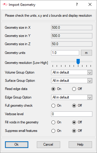
Figure 9.For this tutorial, the default values for the Import Geometry dialog are used to load the geometry. If you have previously used AcuConsole, be sure that any settings that you might have altered are manually changed to match the default values shown in the figure. With the default settings, volumes from the CAD model are added to a default volume group. Surfaces from the CAD model are added to a default surface group. You will work with groups later in this tutorial to create new groups, set flow parameters, add geometric components, and set meshing parameters.
-
Rotate and zoom in the visualization to view the entire model.

Figure 10.The color of objects shown in the modeling window in this tutorial and those displayed on your screen may differ. The default color scheme in AcuConsole is "random," in which colors are randomly assigned to groups as they are created. In addition, this tutorial was developed on Windows. If you are running this tutorial on a different operating system, you may notice a slight difference between the images displayed on your screen and the images shown in the tutorial.
Create a Volume Group and Apply Volume Parameters
Volume groups are containers used for storing information about volumes. This information includes the list of geometric volumes associated with the container, as well as parameters such as material models and mesh sizing information.
When the geometry was imported into AcuConsole, all volumes were placed into the default volume container.
In the next steps you will rename the default group to Fluid, set the material for that group and add the volume from the geometry to that volume group.
-
Toggle the display of the default volume container by clicking
 and
and  next
to the volume name.
Note: You may not see any change when toggling the display if Surfaces are being displayed, as surfaces and volumes may overlap.
next
to the volume name.
Note: You may not see any change when toggling the display if Surfaces are being displayed, as surfaces and volumes may overlap. -
Ensure that the Material model is set to Air.
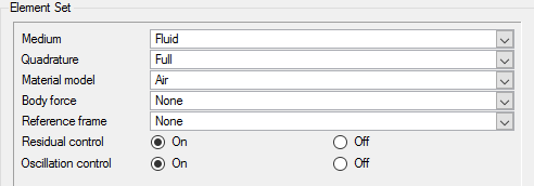
Figure 11.
Create Surface Groups and Apply Surface Parameters
Surface groups are containers used for storing information about a surface. This information includes the list of geometric surfaces associated with the container, as well as parameters such as boundary conditions, surface outputs and mesh sizing information.
In the next steps you will define surface groups, assign the appropriate parameters for each group in the problem and add surfaces to the groups.
Set Farfield Boundary Conditions
In the next steps you will define a surface group for the farfield boundary, set the inlet velocity and add the corresponding surface from the geometry to this group.
-
Select the edge surface in the visualization window (highlighted in gray below)
and then select Done.
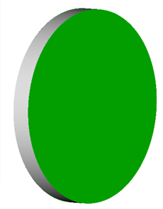
Figure 12. -
Set Turbulence intensity type to Auto.
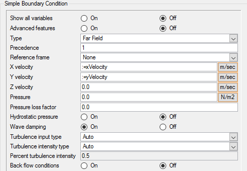
Figure 13.You can see the value of Percent turbulence intensity is set to 0.5. This value is automatically selected by AcuConsole based on parameters like the turbulence model selected, flow type, etc.
Set Remaining Boundary Conditions
In the next steps you will define surface groups for slip and wall boundaries.
-
Select the edge surface in the visualization window (highlighted in gray below)
and then select Done.
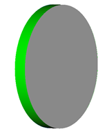
Figure 14. -
Select the edge surface in the visualization window (highlighted in gray below)
and then select Done.
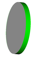
Figure 15. -
Select the edge surface in the visualization window (shown below) and then
select Done.
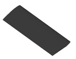
Figure 16.
Define Nodal Initial Conditions
In the next steps you will define the nodal initial conditions.
For the SST and K-Omega turbulence models, you need to enter the initial values for Kinetic energy and Eddy frequency. If you have a reasonable estimate of these values, you can enter them directly in the fields. One option is to use the same values that are assigned at the inlet boundary. In the absence of good estimates for the initial conditions, it is also possible to let AcuSolve perform an automatic initialization of the turbulence variables. By leaving these values set to zero, AcuSolve will trigger an automatic initialization of these variables.
-
Set the Kinetic energy and Eddy frequency to 0.0 to
trigger the automatic initialization.
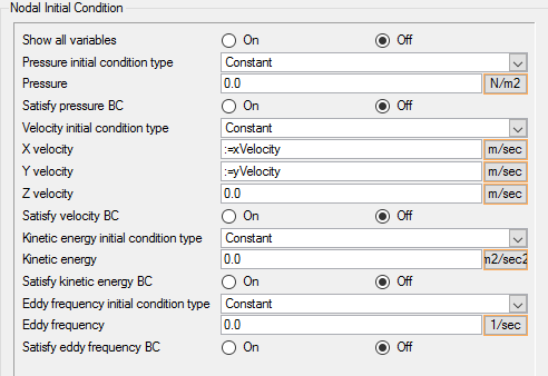
Figure 17.
Assign Mesh Controls
Set Global Meshing Parameters
Now that the simulation has been defined, parameters need to be added to define the mesh sizes that will be created by the mesher.
- Global mesh controls apply to the whole model without being tied to any geometric component of the model.
- Zone mesh controls apply to a defined region of the model, but are not associated with a particular geometric component.
- Geometric mesh controls are applied to a specific geometric component. These controls can be applied to volume groups, surface groups or edge groups.
-
Set Maximum sweep angle to :=sweepAngle.
This setting instructs the mesher to use the sweepAngle parameter to define the maximum angle between radial element lines when creating radial edge blends during the boundary layer meshing process.
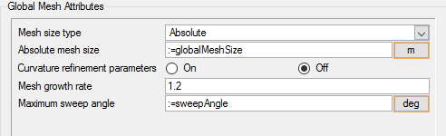
Figure 18.
Set Mesh Process Parameters
- Locally reduce the number of layers in the boundary layer stack to maintain high quality boundary layer elements.
- Locally reduce the height of the boundary layer stack, but keep the total number of layers constant. Using this approach, the height of each layer is scaled by a constant factor to reduce the total height of the stack and avoid the creation of the poor quality boundary layer elements.
-
Set the 2D Boundary layer adjacent height smoothing ratio to
0.25.
This parameter controls how smoothly the local boundary layer heights vary from one element to the next after the layers height are adjusted locally to resolve poor quality elements. A low value of this parameter smooths the variation in height over a large distance, while a value closer to 1.0 enforces a more abrupt change in height. Note that there are separate values of this setting for 2D and 3D boundary layers. For this application, you will be creating a 2D mesh and extruding it in the third direction to create the volume. Therefore, the 2D setting will control the behavior of the mesh in this case.
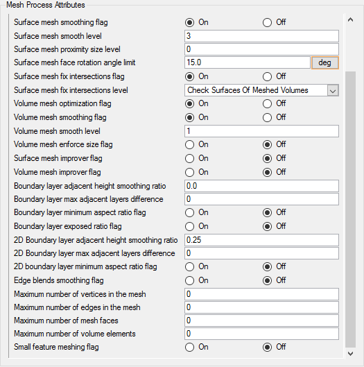
Figure 19.
Set Surface Mesh Parameters
The surface mesh size on the airfoil is controlled through a combination of the mesh size set on the perimeter edges of the airfoil and the mesh size applied directly to the surface. In this tutorial you will also use the region of influence option of the surface mesh to create a refined mesh at a specified distance from the airfoil surface.
-
For Maximum sweep angle, enter :=sweepAngle.
With these settings, the boundary layer mesher will create radial edge blends with a maximum angle defined by the sweepAngle variable.
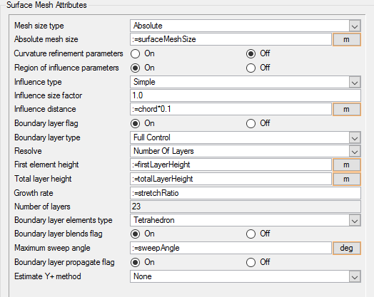
Figure 20.
Set Edge Mesh Parameters
To create an optimum mesh on the surface of the airfoil, it is necessary to have high levels of refinement near the leading and trailing edges and a large element size near the mid chord. Since the surface mesh size was set to constant to serve as the size that is propagated into the volume for the region of influence refinement, you will use an edge mesh parameter to control the placement of nodes along the airfoil surface. To accomplish this, you will first need to create an edge group that contains the perimeter edges of the airfoil.
-
Select the two perimeter edges of the airfoil to add them to this group.
-
Select the two perimeter edges of the airfoil shown below.
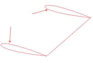
Figure 21.
-
Select the two perimeter edges of the airfoil shown below.
-
Set the Mesh size type to Absolute Expression.
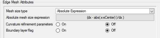
Figure 22. -
Enter the following expression:
sizeMin  = 0.0025
sizeMax = 0.1

xMin =(0.0)
xMax =(1.0)

xCenter =((xMin+xMax)/2.0)
dx = ((xMax-xMin)/2.0)

fac = ((dx - abs(x-xCenter) )/dx )

power = (ln(sizeMax/sizeMin))
expVal = sizeMin*exp(power*fac)

linVal = sizeMin+(sizeMax-sizeMin)*fac

value = expVal
This expression takes the min and max surface mesh size (sizeMin and sizeMax) along with the location of the leading and trailing edge (xMin and xMax) and computes a logarithmic expansion of the surface mesh size as a function of distance from the leading and trailing edges. The mesh size at the leading and trailing edge corresponds to sizeMin and the size at the mid chord location corresponds to sizeMax.
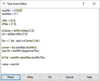
Figure 23.
Set Mesh Extrusion Parameters
The final step in the setup of the meshing for the airfoil is the creation of a mesh extrusion attribute. This extrusion will be defined such that a single element is created across the span of the airfoil.
-
Click OK to accept these settings.
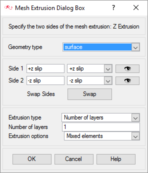
Figure 24.
Generate the Mesh
In the next steps you will generate the mesh that will be used when computing a solution for the problem.
-
Click
 on the toolbar to open the Launch
AcuMeshSim dialog.
on the toolbar to open the Launch
AcuMeshSim dialog.
-
Zoom in on the trailing edge of the airfoil to see the impact of setting the
boundary layer blends flag to on. The radial edge blend at the trailing edge of
the airfoil is clearly evident.
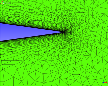
Figure 25.
Compute the Solution and Review the Results
Run AcuSolve and Examine the .log File
In the next steps, you will launch AcuSolve to compute the solution for this case.
-
Click
 on the toolbar to open the
Launch AcuSolve dialog.
on the toolbar to open the
Launch AcuSolve dialog.
-
Once the analysis is complete, scroll up to the top of the file and look for
the message about initializing turbulence field values.
This is because the nodal initial conditions were set to 0. Notice that it reports the min, max and average values of the initialized variables.
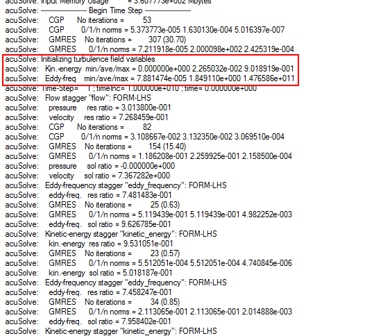
Figure 26. -
Review a single time step.
One thing to notice is that eddy frequency and kinetic energy are solved for three times in each time step. This is the most efficient way to get a converged solution when using the SST and k-omega turbulence models.
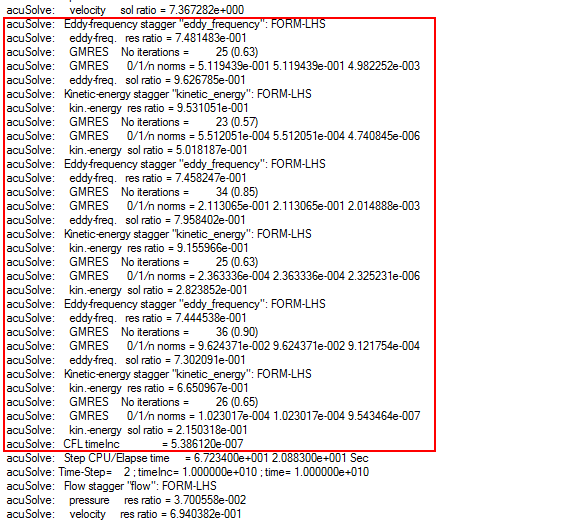
Figure 27.
Monitor the Solution with AcuProbe
While AcuSolve is running, you can monitor the kinetic energy using AcuProbe.
-
Open AcuProbe by clicking
 on the toolbar.
-
Right-click kinetic_energy and select
Plot.
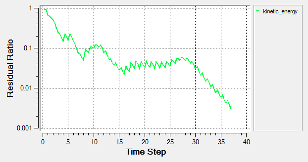
Figure 28. -
Right-click on Final and select Plot
All.
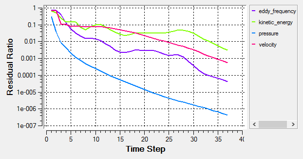
Figure 29.
Start AcuFieldView
-
Click
 on the
AcuConsole toolbar to open the
Launch AcuFieldView dialog.
on the
AcuConsole toolbar to open the
Launch AcuFieldView dialog.
Display Square Root of the Eddy Period
In the next steps you will create a boundary surface to display contours of a new variable, called the square root of the eddy period. When solving for the SST and k-omega turbulence models, AcuSolve introduces three new variables to the output; kinetic_energy (k), eddy_frequency (ω) and sqrt_eddy_per ( ). The sqrt_eddy_per variable is useful for visualizing the turbulent time scale since the eddy_frequency variable has such a large range of values, it is often times easier to visualize sqrt_eddy_per.
These steps are provided with the assumption that you are able to manipulate the view in AcuFieldView. If you are unfamiliar with basic AcuFieldView operations, refer to Manipulate the Model View in AcuFieldView.
-
Click
 on the side toolbar to open the
Boundary Surface dialog.
Note: The dialog may already be open. This step will put the focus on the dialog.
on the side toolbar to open the
Boundary Surface dialog.
Note: The dialog may already be open. This step will put the focus on the dialog. -
Select sqrt_eddy_period and then select
Calculate.
Note: You may have to scroll down to find sqrt_eddy_period. This is a new variable and it represents one over the square root of omega. It has been added as it is a more well bounded variable to plot, as compared to the eddy frequency.
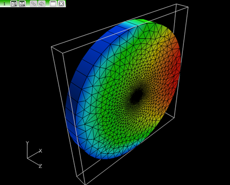
Figure 30. -
Zoom into the airfoil to view the sqrt_eddy_period around the airfoil.
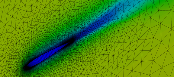
Figure 31.
Post-Process to Calculate Flow Coefficients
AcuSolve is shipped with a number of utility scripts to facilitate the pre and post-processing of a problem solved using the solver. You will be introduced to two of these scripts, AcuLiftDrag and AcuGetCpCf in this section, and their usage. These two scripts are focused on aerodynamic simulations as the ones solved in this tutorial.
Run AcuLiftDrag
AcuLiftDrag is a utility script used to calculate the lift and drag coefficients for an airfoil.
In the Analyze the Problem section, it was described that the simulation is performed as 2D by including only a single layer of extruded elements in the airfoil span direction. When solving a problem in such a way, the span of the airfoil should be set equal to the thickness of the domain in the extrusion direction. When solving a 3D problem, the actual span of the airfoil should be used.
To execute the AcuLiftDrag script for this position, follow the steps below:
-
Enter the following command at the prompt:
acuLiftDrag -osis airfoil -aoa 5 -ref_vel 14.54 -chord 1 -rho 1.225
-span 50
The output of the command should look like the image below: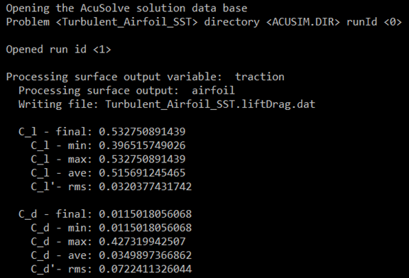
Figure 32.The value C_l corresponds to the lift coefficient, and C_d corresponds to the drag coefficient. The final keyword refers to the respective coefficient values at the last time step of the simulation. The rest of the values provide the basic statistics for these coefficients over all the time steps of the simulation. These statistics are more meaningful if the simulation is transient.
The script also creates the file Turbulent_Airfoil_SST.liftDrag.dat in the problem directory. The file contains the lift and drag data for all the available time steps in a determined tabular arrangement. The first column is the time step, the second column is the lift coefficient, and the third column is the drag coefficient.
Run AcuGetCpCf
AcuGetCpCf is another utility script used to calculate the pressure coefficient (Cp) for the airfoil.
To execute the AcuGetCpCf script for this problem, follow the steps below:
-
Enter the following command at the prompt:
acuGetCpCf -osis airfoil -type cp -ref_vel 14.54 -rho
1.225 -no_nc
The output of the command should look like the image below:
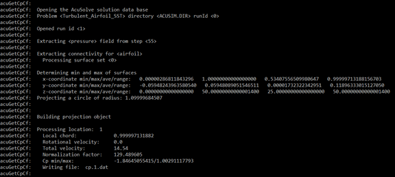
Figure 33.The script prints the minimum and maximum values for the pressure coefficient. It also creates a file, cp.1.dat, in the problem directory. The file contains the pressure coefficient data along the chord of the airfoil. The first column is the x-coordinate along the chord, and the second column is the pressure coefficient. You can use an external plotting utility to the plot the data. The resulting plot is shown below.
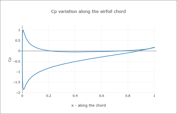
Figure 34.
Change the Angle of Attack and Compute the Solution
Because this database was set up using variables and expressions, it is easy to re-run the simulation again using a different angle of attack. To accomplish this, open the Variable Manager, and set “alpha” to 0.0. Because the xVelocity and yVelocity variables that were defined for the initial and boundary conditions are a function of this parameter, the database will automatically be updated to reflect the new settings. You can simply write the input again and run the solver to obtain a different angle of attack solution.