ACU-T: 2000 Turbulent Flow in a Mixing Elbow
Prerequisites
Prior to starting this tutorial, you should have already run through the introductory HyperWorks tutorial, ACU-T: 1000 HyperWorks UI Introduction. To run this simulation, you will need access to a licensed version of HyperWorks CFD and AcuSolve.
Prior to running through this tutorial, copy HyperWorksCFD_tutorial_inputs.zip from <Altair_installation_directory>\hwcfdsolvers\acusolve\win64\model_files\tutorials\AcuSolve to a local directory. Extract ACU-T2000_MixingElbow.hm from HyperWorksCFD_tutorial_inputs.zip.
Problem Description
The problem to be addressed in this tutorial is shown schematically in Figure 1. This is a typical industrial example for mixing in a pipe by injecting high-velocity fluid from a small inlet into relatively low-velocity fluid in the main pipe. It consists of a 90° mixing elbow with water entering through two inlets with different velocities. The geometry is symmetric about the XY midplane of the pipe, as shown in the figure.

Figure 1. Schematic of Mixing Elbow
Start HyperWorks CFD and Open the HyperMesh Database
-
From the Home tools, Files tool group, click the Open Model tool.

Figure 2.The Open File dialog opens.
Validate the Geometry
-
From the Geometry ribbon, click the Validate tool.

Figure 3.The Validate tool scans through the entire model, performs checks on the surfaces and solids, and flags any defects in the geometry, such as free edges, closed shells, intersections, duplicates, and slivers.The current model doesn’t have any of the issues mentioned above. Alternatively, if any issues are found, they are indicated by the number in the brackets adjacent to the tool name.
Observe that a blue check mark appears on the top-left corner of the Validate icon. This indicates that the tool found no issues with the geometry model.
Figure 4.
Set Up the Problem
Set Up the Simulation Parameters and Solver Settings
-
From the Flow ribbon, click the Physics tool.

Figure 5.The Setup dialog opens. -
Under the Physics models setting:
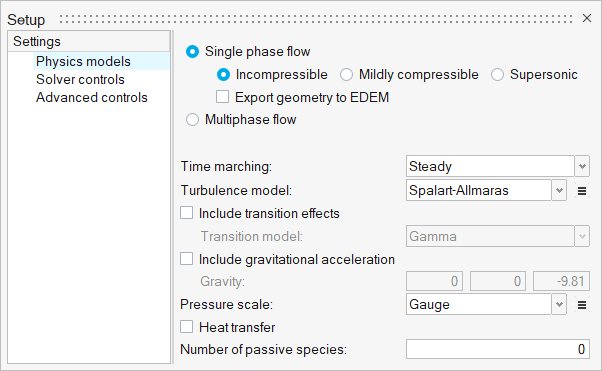
Figure 6. -
Click the Solver controls setting and verify that the
parameters are set as shown in the figure below.
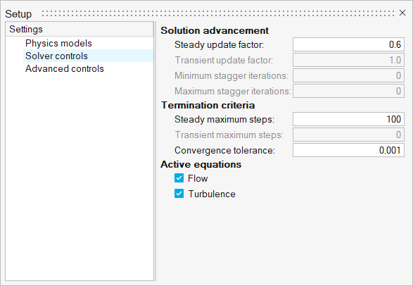
Figure 7.
Assign Material Properties
-
From the Flow ribbon, click the Material tool.

Figure 8. -
Select the model body.
The entire solid is highlighted.
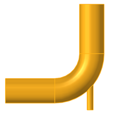
Figure 9. -
On the guide bar, click
 to execute
the command and exit the tool.
to execute
the command and exit the tool.
Assign Flow Boundary Conditions
Set Boundary Conditions for the Large Inlet
-
From the Flow ribbon, Profiled
tool group, click the Profiled Inlet tool.

Figure 10. -
Click the face of the large inlet.
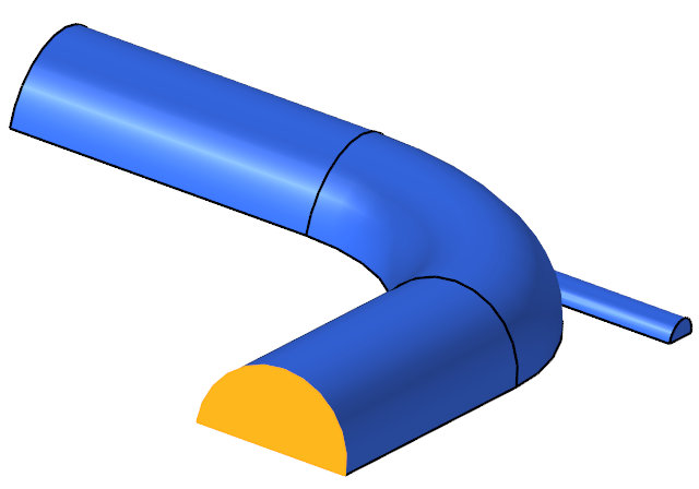
Figure 11. -
In the microdialog, enter a value of
0.4 for Average velocity.
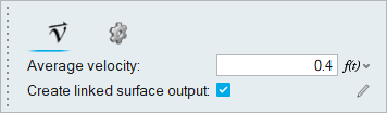
Figure 12. -
On the guide bar, click
 to execute the command and remain in the
tool.
Note: The number of inlets created appears in parenthesis on the top-right of the Profiled tool icon.
to execute the command and remain in the
tool.
Note: The number of inlets created appears in parenthesis on the top-right of the Profiled tool icon.
Set Boundary Conditions for the Small Inlet
-
Click the face of the small inlet.
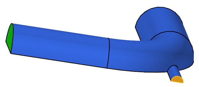
Figure 13. -
In the microdialog, enter a value of
1.2 for Average velocity.
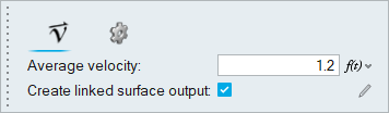
Figure 14. -
On the guide bar, click
to execute
the command and exit the tool.
Set Boundary Conditions for the Outlet
-
From the Flow ribbon, click the Outlet tool.

Figure 15. -
Click the face of the outlet.
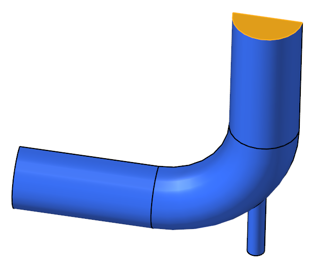
Figure 16. -
In the microdialog, make sure both
Static pressure and Pressure loss factor are 0.
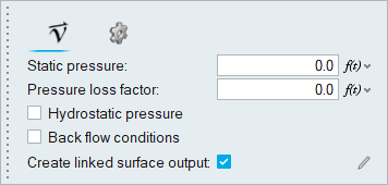
Figure 17. -
On the guide bar, click
to execute
the command and exit the tool.
Set Boundary Conditions for the Symmetry Plane
This geometry is symmetric about the XY midplane, and can therefore be modeled with half of the geometry. In order to take advantage of this, the midplane needs to be identified as a symmetry plane. The symmetry boundary condition enforces constraints such that the flow field from one side of the plane is a mirror image of that on the other side.
-
From the Flow ribbon, click the Symmetry tool.

Figure 18. -
Select the face of the symmetry plane.
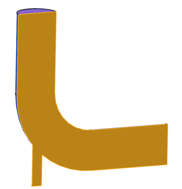
Figure 19. -
In the microdialog, accept the
default symmetry conditions.
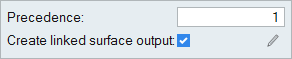
Figure 20. -
On the guide bar, click
to execute
the command and exit the tool.
Generate the Mesh
-
From the Mesh ribbon, click the
Volume tool.

Figure 21.The Meshing Operations dialog opens.Note: If the model has not been validated, you are prompted to create the simulation model before running the batch mesh. -
Accept all other default parameters.
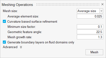
Figure 22. -
From the back side of the model, observe the refined mesh around the small
inlet.
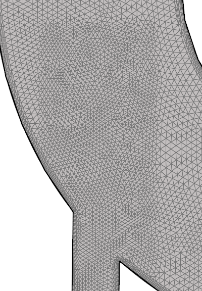
Figure 23.
Run AcuSolve
-
From the Solution ribbon, click the Run tool.

Figure 24.The Launch AcuSolve dialog opens. -
Leave the remaining options as default and click
Run to launch AcuSolve.
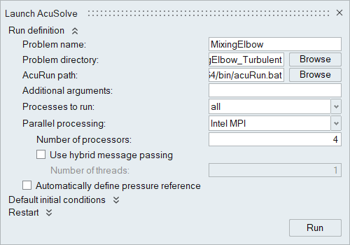
Figure 25.The Run Status dialog opens. Once the run is complete, the status is updated and you can close the dialog.Tip: While AcuSolve is running, right-click on the AcuSolve job in the Run Status dialog and select View Log File to monitor the solution process.
Post-Process the Results with HW-CFD Post
-
Click
 and set the Colormap Name to Rainbow
Uniform.
and set the Colormap Name to Rainbow
Uniform.
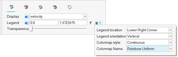
Figure 26. -
Click
 on the guide bar.
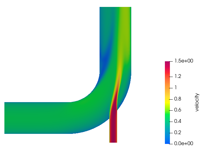
Figure 27. -
Click
 to reset the range.
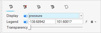
Figure 28. -
Click on the guide bar.
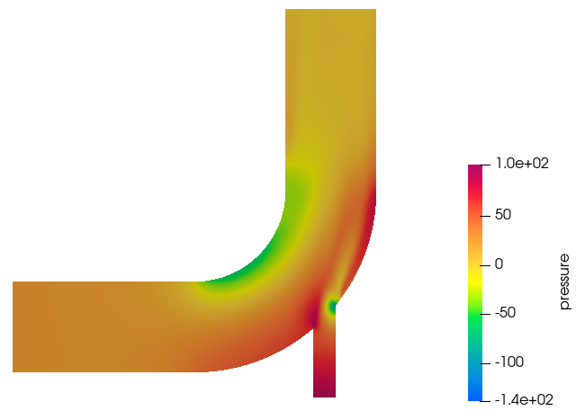
Figure 29.
Summary
In this tutorial, you worked through a basic workflow to set up a CFD model, carry out a CFD simulation, and post-process the results. You started by importing the model in HyperWorks CFD. Then, you defined the simulation parameters and launched AcuSolve directly from within HyperWorks CFD. Upon completion of the solution by AcuSolve, you used the Post ribbon to create contour plots.