ELEMENT_BOUNDARY_CONDITION
Specifies an element boundary condition for a solution field on a set of element faces.
Type
AcuSolve Command
Syntax
ELEMENT_BOUNDARY_CONDITION("name") {parameters...}
Qualifier
User-given name.
Parameters
- shape (enumerated) [no default]
- Shape of the surfaces in this set.
- three_node_triangle or tri3
- Three-node triangle.
- four_node_quad or quad4
- Four-node quadrilateral
- six_node_triangle or tri6
- Six-node triangle.
- element_set or elem_set (string) [no default]
- User-given name of the parent element set.
- surfaces (array) [no default]
- List of element surfaces.
- surface_sets (list) [={}]
- List of surface set names (strings) to use in this element boundary condition. When using this option, the connectivity, shape, and parent element of the surfaces are provided by the surface set container and it is unnecessary to specify the shape, element_set and surfaces parameters directly to the ELEMENT_BOUNDARY_CONDITION command. This option is used in place of directly specifying these parameters. In the event that both of the surface_sets and surfaces parameters are provided, the full collection of surface elements is read and a warning message is issued. The surface_sets option is the preferred method to specify the surface elements. This option provides support for mixed element topologies and simplifies pre-processing and post-processing.
- variable or var (enumerated) [no default]
- Boundary condition variable. All are scalars except tangential_traction is
a three-component vector.
- mass_flux or mass
- Mass flux (mass flow rate).
- pressure or pres
- Pressure.
- stagnation_pressure or stag_pres
- Stagnation pressure.
- tangential_traction or trac
- Tangential components of traction.
- heat_flux or heat
- Thermal heat flux.
- convective_heat_flux or conv_heat
- Convective heat flux.
- radiation_heat_flux or rad_heat
- Radiation heat flux.
- species_1_flux or spec1
- Species 1 flux.
- convective_species_1_flux or conv_spec1
- Convective flux for species 1.
- species_2_flux or spec2
- Species 2 flux.
- convective_species_2_flux or conv_spec2
- Convective flux for species 2.
- species_3_flux or spec3
- Species 3 flux.
- convective_species_3_flux or conv_spec3
- Convective flux for species 3.
- species_4_flux or spec4
- Species 4 flux.
- convective_species_4_flux or conv_spec4
- Convective flux for species 4.
- species_5_flux or spec5
- Species 5 flux.
- convective_species_5_flux or conv_spec5
- Convective flux for species 5.
- species_6_flux or spec6
- Species 6 flux.
- convective_species_6_flux or conv_spec6
- Convective flux for species 6.
- species_7_flux or spec7
- Species 7 flux.
- convective_species_7_flux or conv_spec7
- Convective flux for species 7.
- species_8_flux or spec8
- Species 8 flux.
- convective_species_8_flux or conv_spec8
- Convective flux for species 8.
- species_9_flux or spec9
- Species 9 flux.
- convective_species_9_flux or conv_spec9
- Convective flux for species 9.
- field_flux or field
- Multi field flux.
- convective_field_flux or conv_field
- Multi field convective flux.
- turbulence_flux or turb
- Turbulence diffusion flux.
- kinetic_energy_flux or tke
- Turbulence kinetic energy flux.
- dissipation_rate_flux or teps
- Turbulence dissipation rate flux.
- eddy_frequency_flux or tomega
- Turbulence eddy frequency flux.
- intermittency_flux or tintc
- Transition intermittency flux.
- transition_re_theta_flux or treth
- Transition Re-theta flux.
- type (enumerated) [=zero]
- Type of the boundary condition.
- zero
- Zero for the set.
- constant or const
- Constant value. Requires constant_value.
- free
- Computes the boundary values from the solution field.
- outflow or out
- An outflow condition for the mass_flux variable.
- inflow or in
- An inflow condition for the mass_flux variable.
- per_surface or surf
- Surface values. Requires surface_values.
- piecewise_linear or linear
- Piecewise linear curve fit. Requires curve_fit_values and curve_fit_variable.
- cubic_spline or spline
- Cubic spline curve fit. Requires curve_fit_values and curve_fit_variable.
- user_function or user
- User-defined function. Requires user_function, user_values and user_strings.
- constant_value or value (real) [=0]
- Constant scalar value of the boundary condition. Used with constant type and scalar variables.
- constant_values (array) [={0,0,0}]
- Constant vector value of the boundary condition. Used with constant type and vector variables (currently only tangential_traction).
- field (string) [no default]
- Value of the boundary condition for field. Used with variable field.
- surface_values or values (array) [no default]
- A two-column (for scalar variables) or four-column (for vector variables, currently only tangential_traction) array of surface/boundary-condition data values. Used with per_surface type.
- curve_fit_values or curve_values (array) [={0,0}]
- A two-column (for scalar variables) or four-column (for vector variables, currently only tangential_traction) array of independent-variable/boundary-condition data values. Used with piecewise_linear and cubic_spline types.
- curve_fit_variable or curve_var (enumerated) [=temperature]
- Independent variable of the curve fit. Used with piecewise_linear and
cubic_spline types.
- x_coordinate or xcrd
- X-component of coordinates.
- y_coordinate or ycrd
- Y-component of coordinates.
- z_coordinate or zcrd
- Z-component of coordinates.
- x_reference_coordinate or xrefcrd
- X-component of reference coordinates.
- y_reference_coordinate or yrefcrd
- Y-component of reference coordinates.
- z_reference_coordinate or zrefcrd
- Z-component of reference coordinates.
- x_velocity or xvel
- X-component of velocity.
- y_velocity or yvel
- U-component of velocity.
- z_velocity or zvel
- Z-component of velocity.
- velocity_magnitude or vel_mag
- Velocity magnitude.
- normal_velocity
- Normal velocity.
- pressure or pres
- Pressure.
- temperature or temp
- Temperature.
- relative_humidity
- Relative humidity.
- dewpoint_temperature
- Dewpoint temperature.
- eddy_viscosity or eddy
- Turbulence kinematic eddy viscosity.
- kinetic_energy or tke
- Turbulence kinetic energy.
- dissipation_rate or teps
- Turbulence dissipation rate.
- intermittency or tintc
- Transition intermittency.
- transition_re_theta or treth
- Transition Re-theta.
- eddy_frequency or tomega
- Turbulence eddy frequency.
- species_1 or spec1
- Species 1.
- species_2 or spec2
- Species 2.
- species_3 or spec3
- Species 3.
- species_4 or spec4
- Species 4.
- species_5 or spec5
- Species 5.
- species_6 or spec6
- Species 6.
- species_7 or spec7
- Species 7.
- species_8 or spec8
- Species 8.
- species_9 or spec9
- Species 9.
- mesh_x_displacement or mesh_xdisp
- X-component of mesh displacement.
- mesh_y_displacement or mesh_ydisp
- Y-component of mesh displacement.
- mesh_z_displacement or mesh_zdisp
- Z-component of mesh displacement.
- mesh_displacement_magnitude or mesh_disp_mag
- Mesh displacement magnitude.
- mesh_x_velocity or mesh_xvel
- X-component of mesh velocity.
- mesh_y_velocity or mesh_yvel
- Y-component of mesh velocity.
- mesh_z_velocity or mesh_zvel
- Z-component of mesh velocity.
- mesh_velocity_magnitude or mesh_vel_mag
- Mesh velocity magnitude.
- user_function or user (string) [no default]
- Name of the user-defined function. Used with user_function type.
- user_values (array) [={}]
- Array of values to be passed to the user-defined function. Used with user_function type.
- user_strings (list) [={}]
- Array of strings to be passed to the user-defined function. Used with user_function type.
- multiplier_function (string) [=none]
- User-given name of the multiplier function for scaling the boundary condition values. If none, no scaling is performed.
- reference_temperature or ref_temp (real) [=273.15]
- Reference temperature for the convective and radiation heat flux boundary conditions
- reference_temperature_multiplier_function (string) [=none]
- User-given name of the multiplier function for scaling the reference temperature. If none, no scaling is performed.
- reference_species or ref_spec (real) [=0]
- Reference species for the convective species boundary condition.
- reference_species_multiplier_function (string) [=none]
- User-given name of the multiplier function for scaling the reference species. If none, no scaling is performed.
- non_reflecting_factor (real) >=0 [=0]
- Amount of non-reflecting modification. If zero, there is no effect. If one, waves can pass through the boundary without reflection. Used with pressure variable at outflow boundaries and mass_flux variable at inflows. Turning on both non_reflecting_bc_running_average_field and running_average specifies the use of running average fields to enhance the performance of non-reflective boundary conditions when flow = navier_stokes is used. When flow = compressible_navier_stokes is set, the running_average option does not need to be turned on.
- pressure_loss_factor (real) >=0 [=0]
- Coefficient of a pressure loss term added/subtracted to outflow/inflow pressure boundary conditions. Used with pressure variable.
- pressure_loss_factor_multiplier_function (string) [=none]
- User-given name of the multiplier function for scaling the pressure loss factor. Used with pressure variable. If none, no scaling is performed.
- hydrostatic_pressure (boolean) [=off]
- Flag specifying whether to add hydrostatic pressure to pressure and stagnation pressure boundary conditions.
- hydrostatic_pressure_origin (array) [={0,0,0}]
- Coordinates of any location where the hydrostatic pressure is zero. Used with hydrostatic_pressure=on, and pressure and stagnation pressure boundary conditions.
- active_type (enumerated) [=all]
- Type of the active flag. Determines which surfaces in this set will have element boundary
conditions imposed by this command.
- all
- All surfaces in this set are active.
- none
- No surfaces in this set are active.
- no_interface
- Only surfaces that are not in an interface surface set or do not find a contact surface of an appropriate medium are active.
Description
ELEMENT_SET( "flow elements" ) {
    shape           = four_node_tet
    elements        = { ...
                        4, 2, 5, 6, 8 ;
                        5, 2, 6, 3, 5 ;
                        ... }
...
}
ELEMENT_BOUNDARY_CONDITION( "constant BC on heated wall" ) {
    shape           = three_node_triangle
    element_set     = "flow elements"
    surfaces        = { 4, 41, 2, 5, 6 ;
                        5, 51, 5, 6, 3 ; }
    variable        = heat_flux
    type            = constant
    constant_value  = 12.
}
defines a thermal heat flux element boundary condition, with a constant value of 12 on two surfaces of the element set "flow elements".
- Element Shape
- Surface Shape
- four_node_tet
- three_node_triangle
- five_node_pyramid
- three_node_triangle
- five_node_pyramid
- four_node_quad
- six_node_wedge
- four_node_quad
- eight_node_brick
- four_node_quad
- ten_node_tet
- six_node_triangle
The surfaces parameter contains the faces of the element set. This parameter is a multi-column array. The number of columns depends on the shape of the surface. For three_node_triangle, this parameter has five columns, corresponding to the element number (of the parent element set), a unique (within this set) surface number, and the three nodes of the element face. For four_node_quad, surfaces has six columns, corresponding to the element number, a surface number, and the four nodes of the element face. For six_node_triangle, surfaces has eight columns, corresponding to the element number, a surface number, and the six nodes of the element face. One row per surface must be given. The three, four, or six nodes of the surface may be in any arbitrary order, since they are reordered internally based on the parent element definition.
4 41 2 5 6
5 51 5 6 3ELEMENT_BOUNDARY_CONDITION( "constant BC on heated wall" ) {
shape = three_node_triangle
element_set = "flow elements"
surfaces = Read( "heated_wall.ebc" )
variable = heat_flux
type = constant
constant_value = 12.
}SURFACE_SET( "tri faces" ) {
surfaces = { 1, 1, 1, 2, 4 ;
2, 2, 3, 4, 6 ;
3, 3, 5, 6, 8 ; }
shape = three_node_triangle
volume_set = "tetrahedra"
}
SURFACE_SET( "quad faces" ) {
surfaces = { 1, 1, 1, 2, 4, 9 ;
2, 2, 3, 4, 6, 12 ;
3, 3, 5, 6, 8, 15 ; }
shape = four_node_quad
volume_set = "prisms"ELEMENT_BOUNDARY_CONDITION ("constant BC on heated wall") {
surface_sets = {"tri_faces", "quad_faces"}
...
}tri faces
quad facesELEMENT_BOUNDARY_CONDITION ("constant BC on heated wall") {
surface_sets = Read("surface_sets.srfst")
...
}The mixed topology version of the ELEMENT_BOUNDARY_CONDITION command is preferred. This version provides support for multiple element topologies within a single instance of the command and simplifies pre-processing and post-processing. In the event that both the surface_sets and surfaces parameters are provided in the same instance of the command, the full collection of surface elements is read and a warning message is issued. Although the single and mixed topology formats of the commands can be combined, it is strongly recommended that they are not.
The variable to which the boundary condition applies is given by variable. If the problem does not solve for a field associated with this variable, the boundary condition is simply ignored.
The element boundary conditions are applied at the quadrature points of the surfaces. The quadrature rule is inherited from the parent element set of the surface.
A constant boundary condition applies the same boundary condition for all quadrature points of the surfaces, as in the above example.
ELEMENT_BOUNDARY_CONDITION( "constant BC on outflow pressure" ) {
 surface_sets = {"tri_faces", "quad_faces"}
 variable     = pressure
 type         = zero
}ELEMENT_BOUNDARY_CONDITION( "outflow traction" ) {
surface_sets = {"tri_faces", "quad_faces"}
variable = tangential_traction
type = free
}On boundary surfaces where no element boundary condition is specified for the mass_flux variable, one is added of type free. The same is done for the pressure variable. For all other variables nothing is added (which is the same as adding an element boundary condition of type zero). Note that outflow and free surfaces normally require a pressure boundary condition of type zero (or constant). These must be specified. The free type is not available for convective and radiation type variables.
ELEMENT_BOUNDARY_CONDITION( "outflow mass flux" ) {
 surface_sets = {"tri_faces", "quad_faces"}
 variable     = mass_flux
 type         = outflow
}ELEMENT_BOUNDARY_CONDITION( "per surface BC on heated wall" ) {
shape = three_node_triangle
element_set = "flow elements"
surfaces = { 4, 41, 2, 5, 6 ;
5, 51, 5, 6, 3 ; }
variable = heat_flux
type = per_surface
surface_values = { 41, 2 ;
51, 4 ; }
}For scalar variables, the surface_values parameter is a two-column array corresponding to the surface number and boundary condition values. For vector variables (currently only tangential_traction), surface_values is a four-column array corresponding to the surface number and the xyz components of the boundary condition. The surface numbers must match those given by surfaces. No surface may be missing.
41 2
51 4ELEMENT_BOUNDARY_CONDITION( "per surface BC on heated wall" ) {
shape = three_node_triangle
element_set = "flow elements"
surfaces = Read( "heated_wall.ebc" )
variable = heat_flux
type = per_surface
surface_values = Read( "heated_wall.heat" )
}The per_surface option is currently not supported with mixed topology input.
ELEMENT_BOUNDARY_CONDITION( "curve fit BC on convective heat wall" ) {
 surface_sets          = {"tri_faces", "quad_faces"}
 variable              = convective_heat_flux
 type                  = piecewise_linear
 curve_fit_values      = { 0, 0.0 ;
                          10, 1.5 ; }
 curve_fit_variable    = x_coordinate
 reference_temperature = 25
}
defines a convective heat transfer boundary condition as a function of the x-coordinates. In this example the convective heat coefficient varies linearly from h = 0 at x = 0 to h = 1.5 at x = 10. For scalar variables the curve_fit_values parameter is a two-column array corresponding to the independent variable and the boundary condition values. For vector variables, currently only tangential_traction, curve_fit_values is a four-column array corresponding to the independent variable and the xyz components of the boundary condition. The independent variable values must be in ascending order. The limit point values of the curve fit are used when curve_fit_variable falls outside of the curve fit limits. The curve fit variable nornal_velocity is positive when the flow goes out of the parent element.
0 0.0
10 1.5ELEMENT_BOUNDARY_CONDITION( "curve fit BC on convective heat wall" ) {
surface_sets = {"tri_faces", "quad_faces"}
variable = convective_heat_flux
type = piecewise_linear
curve_fit_values = Read( "conv_wall.fit" )
curve_fit_variable = x_coordinate
reference_temperature = 25
}An element boundary condition of type user_function may be used to model more complex behaviors; see the AcuSolve User-Defined Functions Manual for a detailed description of user-defined functions.
ELEMENT_BOUNDARY_CONDITION( "UDF BC on inflow pressure" ) {
 surface_sets  = {"tri_faces", "quad_faces"}
 variable      = pressure
 type          = user_function
 user_function = "usrElementBcExample"
 user_values   = { 100,      # pressure
                     1.225 } # density
}#include "acusim.h"
#include "udf.h"
UDF_PROTOTYPE( usrElementBcExample ) ; /* function prototype */
Void usrElementBcExample (
UdfHd udfHd, /* Opaque handle for accessing data */
Real* outVec, /* Output vector */
Integer nItems, /* Number of BC surfaces */
Integer vecDim /* = 1 */
) {
Integer surf ; /* a surface counter */
Real dens ; /* density */
Real stagPres ; /* stagnation pressure */
Real velSqr ; /* velocity square */
Real* usrVals ; /* user values */
Real* vel ; /* velocity */
Real* xVel ; /* x-component of velocity */
Real* yVel ; /* y-component of velocity */
Real* zVel ; /* z-component of velocity */
udfCheckNumUsrVals( udfHd, 2 ) ; /* check for error */
usrVals = udfGetUsrVals( udfHd ) ; /* get the user vals */
stagPres = usrVals[0] ; /* get BC value */
dens = usrVals[1] ; /* get density */
vel = udfGetEbcData( udfHd, UDF_EBC_VELOCITY ) ; /* get the velocity */
xVel = &vel[0*nItems] ; /* localize x-vel. */
yVel = &vel[1*nItems] ; /* localize y-vel. */
zVel = &vel[2*nItems] ; /* localize z-vel. */
for ( surf = 0 ; surf < nItems ; surf++ ) {
velSqr = xVel[surf] * xVel[surf]
+ yVel[surf] * yVel[surf]
+ zVel[surf] * zVel[surf] ;
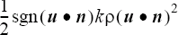
outVec[surf] = stagPres - 0.5 * dens * velSqr ;
}
} /* end of usrElementBcExample() */For scalar variables, the dimension of the returned boundary condition vector, outVec, is the number of surfaces.
For vector variables (currently only tangential_traction), the dimension is the number of surfaces times three, with the surface dimension being "faster" (as it is for the velocity vector in the example).
For the tangential_traction variable, the three components specified are in the global xyz coordinate system. The component normal to the surface is removed before the boundary condition is imposed. Thus, there will be no conflict if a pressure (normal component of traction) element boundary condition is also imposed on the same surfaces.
ELEMENT_BOUNDARY_CONDITION( "constant BC on heat flux" ) {
    surface_sets        = {"tri_faces", "quad_faces"}
    variable            = heat_flux
    type                = constant
    constant_value      = 2.5
    multiplier_function = "time varying"
}
MULTIPLIER_FUNCTION( "time varying" ) {
    type                = piecewise_linear
    curve_fit_values    = { 0, 0.0 ;
                           10, 1.0 ;
                           20, 0.5 ;
                           40, 0.7 ;
                           80, 1.2 ; }
    curve_fit_variable = time
}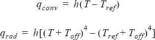
where h is the value of the element boundary condition;
T is the temperature;
Tref is the reference temperature, given by
reference_temperature; and
Toff is the offset to convert to an absolute
temperature, given by the absolute_temperature_offset parameter of the
EQUATION command. For a radiation heat flux boundary condition, the
coefficient may be calculated from  , where
ε is the grey-body emissivity/ absorptivity and σ is the
Stefan-Boltzmann constant. A description of the last two quantities may be found in the
RADIATION command. However, note that the radiation heat flux is specified
independently of the radiation equation and the RADIATION,
RADIATION_SURFACE, and EMISSIVITY_MODEL commands, as well
as the SOLAR_RADIATION and related commands. The convective species fluxes
are defined similarly to the convective heat flux, except that
reference_species is used instead of
reference_temperature.
, where
ε is the grey-body emissivity/ absorptivity and σ is the
Stefan-Boltzmann constant. A description of the last two quantities may be found in the
RADIATION command. However, note that the radiation heat flux is specified
independently of the radiation equation and the RADIATION,
RADIATION_SURFACE, and EMISSIVITY_MODEL commands, as well
as the SOLAR_RADIATION and related commands. The convective species fluxes
are defined similarly to the convective heat flux, except that
reference_species is used instead of
reference_temperature.
ELEMENT_BOUNDARY_CONDITION( "time dependent outside temperature" ) {
    surface_sets                              = {"tri_faces", "quad_faces"}
    variable                                  = convective_heat_flux
    type                                      = constant
    constant_value                            = 12.5
    reference_temperature                     = 1
    reference_temperature_multiplier_function = "outside temperature"
}
MULTIPLIER_FUNCTION( "outside temperature" ) {
    type                                      = cubic_spline
    curve_fit_values                          = { 0*3600, 295 ;
                                                 12*3600, 312 ;
                                                 24*3600, 295 ; }
    curve_fit_variable                        = time
}
Similarly, reference_species_multiplier_function may be used to scale the reference species.
Reflections of waves from inflow and outflow boundaries can be reduced by setting non_reflecting_factor to a positive value. This parameter applies to inflow types with inflow_type = mass_flux and to outflow types. For inflows only the mass flux element boundary condition is modified and for outflows only the pressure element boundary condition is modified. It is ignored for all other cases. Also, there is no effect for the constant density model unless a positive isothermal_compressibility value is specified.
Setting non_reflecting_factor = 0 has no effect; the given element boundary condition is imposed. Using a value of one gives the full effect; waves pass through the boundary without reflection but at the cost of the variable drifting away from its specified value. Other values yield a blend between these effects. Values greater than one for non_reflecting_factor may lead to instabilities for the mass flux condition. If running average fields are defined, that is, running_average = on in the EQUATION command, then an enhanced non-reflecting boundary condition is used, leading to less reflection for the same value of non_reflecting_factor. The non_reflecting_bc_running_average_field needs to be turned on for this option. Note that when flow = compressible_navier_stokes, the running_average option does not need to be turned on; the running average files are automatically used in non- reflecting boundary conditions.
ELEMENT_BOUNDARY_CONDITION( "outflow" ) {
    ...
    variable                                 = pressure
    pressure                                 = 0
    pressure_loss_factor                     = 100
    pressure_loss_factor_multiplier_function = "pLoss_TMF"
    ...
}
MULTIPLIER_FUNCTION( "pLoss_TMF" ) {
    type                                     = piecewise_linear
    curve_fit_values                         = { 1, 1 ;
                                                10 , 0 }
    curve_fit_variable                       = time_step
}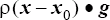
where ρ is the density;
x is the current coordinate vector;
x0 is any coordinate vector where the hydrostatic
pressure is zero, given by hydrostatic_pressure_origin; and
g is the gravity vector given by
body_force in the parent ELEMENT_SET command or is the
gravity_vector given by gravitational_acceleration in
EQUATION. If variable is not
pressure or stagnation_pressure, then
hydrostatic_pressure has no effect. If
multiplier_function is given, it is applied before this term is added. If
gravitational force is modeled using the GRAVITY command, then
hydrostatic_pressure=on should be set for most pressure
or stagnation pressure boundary conditions in order to properly account for the hydrostatic
pressure. This is most commonly needed on outflow boundaries. For free surface pressure
conditions hydrostatic_pressure is normally set to off in
order to ensure that the imposed pressure is constant along the entire surface. If this pressure
or the nominal height of the free surface is nonzero, then
hydrostatic_pressure_origin may be adjusted for any other pressure
boundary condition so that its evaluation at the nominal surface height equals the pressure
imposed on the free surface. That is, 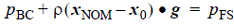 where
where  is a point on
the nominal free surface,
is a point on
the nominal free surface,  is the given
pressure in an ELEMENT_BOUNDARY_CONDITION command with
hydrostatic_pressure=on, and
is the given
pressure in an ELEMENT_BOUNDARY_CONDITION command with
hydrostatic_pressure=on, and  is the given
pressure on the free surface. An example of this adjustment is given in
SIMPLE_BOUNDARY_CONDITION.
is the given
pressure on the free surface. An example of this adjustment is given in
SIMPLE_BOUNDARY_CONDITION.
In some circumstances it is necessary to "turn off" or "deactivate" a previously-defined element boundary condition. This is accomplished by setting the active flag through active_type. A value of all is the default and means that all surfaces in the set are active (active flag = 1) and will have the boundary condition imposed on them. A value of none means that no surface is active (active flag = 0).
- The surface is not in any INTERFACE_SURFACE set; active flag = 1.
- The surface is in an INTERFACE_SURFACE set, but it does not find a contact surface; active flag = 1.
- The surface finds a contact surface of fluid medium; active flag = 0.
- The surface finds a contact surface of solid/shell medium, and variable is defined on the solid/shell side, currently only the heat flux variables,; active flag = 0.
- The surface finds a contact surface of solid/shell medium, and variable is not defined on the solid/shell side, that is, it is not one of the heat flux variables,; active flag = 1.