Setup a frequency response analysis with a series of step-by-step process
templates.
These process templates prompt you to enter generic engineering data, and once the data is
available, automatically create frequency response analysis loadcases and associated solver
cards. The templates share a set of common process steps that are only described the first
time they are used.
Setup a frequency response analysis from the menu bar by
clicking Tools > Freq Resp Process and selecting one of the step-by-step process templates.
Restriction: Only available in the OptiStruct and
Nastran user profiles.
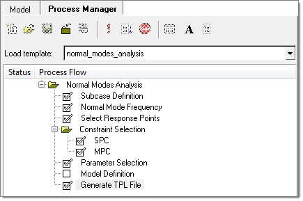
Setup a Normal Model Process
The Normal Modes loadcase Process Manager automatically
generates a loadcase template, which can be used in the Analysis Manager for future
normal modes loadcases without going through the Process Manager again. Figure 1.
From the menu bar, click Tools > Freq Resp Process > Normal Modes.
A normal modes analysis process template is loaded and opens in the Process
Flow browser.
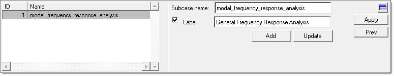
In the Subcase Definition task, create a new subcase or edit an existing
subcase.
Create or edit a subcase.
To create a new subcase, edit the optional subcase label and
click Add.
To edit an existing subcase, highlight an existing subcase in
the list box, edit the optional subcase label and click
Update.
Once input to the task is complete, click Apply to proceed.
Figure 2.
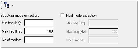
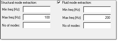
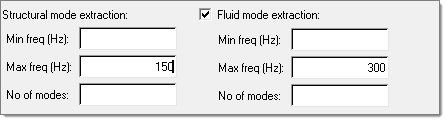
In the Normal Mode Frequency task, define Normal Mode Frequency.
Enter normal modes extraction parameters, such as Min. and Max.
frequency, or the number of modes desired.
In most cases, only input for the Max. frequency field is needed. When
left blank, the Min. frequency is interpreted as 0 (Hz.), and the No. of
modes is however many found between 0 and the Max. frequency. This task
gives you separate control over modal extraction in the structural and
fluid domains.
Once input to the task is complete, click Apply to proceed.
Figure 3.
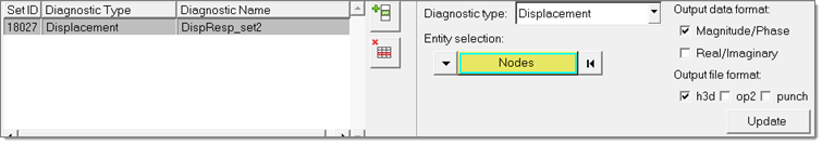
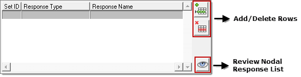
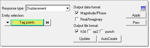
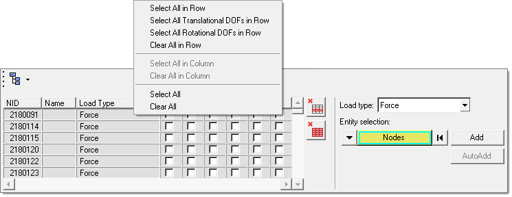
In the Select Response Points task, select response points for output.
Select a Response type, such as Displacement.
Use the Entity selector to select nodes, a node set, or tags to be
included in a particular response set.
You can add or delete multiple response sets from the list using the
Add row and Delete row
icons to the right of the list. Figure 4.
Under Output data format, select the complex frequency response data
format (real/imaginary or magnitude/phase).
Under Output file format, select the output file format (h3d, punch, or
op2).
Once all the required responses have been defined, click
Apply to
proceed.
Figure 5.
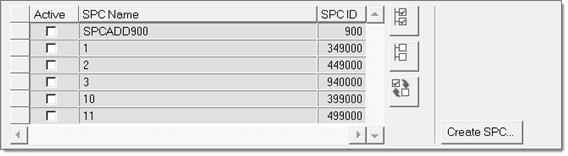
In the Constraint selection, SPC task, select the boundary condition of the
frequency response analysis.
You can select existing SPCs by checking the corresponding box under
the Active column, or click Create SPC to go to
the Constraints panel and define a new SPC.
Once the boundary condition has been fully defined, click
Apply to
proceed.
In the Constraint selection, MPC task, select MPC equations to turn on for the
frequency response analysis.
Select MPCs.
NVH user profile: There are two options for managing MPCs, the
Analysis Manager and the Process Manager. If you select the Analysis Manager, the Select subcase
option and the MPCs list are disabled. If you select the
Process Manager, after you select a
subcase you can then select existing MPCs by checking the
corresponding box under the Active column.
HyperMesh user profile: The Analysis
Manager option is not available, and the MPCs can only be
managed through the Process Manager.
Once the MPC equations have been selected, click Apply to proceed.
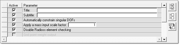
In the Parameter Selection task, select typical solution parameters, such as
title, singular point constraints, and so on.
Check all boxes under the Active column to activate the desired
solution option.
Once the parameters have been selected, click Apply and a Process Manager message box pops up informing you
that the process has come to an end.
Click Yes to close the template, or
No to review or edit the process steps.
Figure 6.
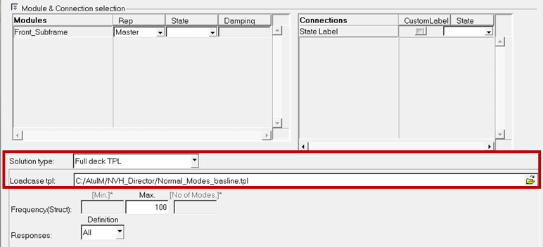
In the Generate TPL file task, generate and save the parameters defined in a
standard template file at your selected location.
In the Analysis Manager, the generated template file can be selected as
loadcase and solver decks can be exported for normal modes analysis. Figure 7.
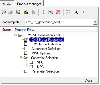
Setup CMS SE Generatin Process
The CMS SE Generation process template helps you generate a CMS SuperElement (SE)
modal model from a finite element based model.
Figure 8.
From the menu bar, click Tools > Freq Resp Process > CMS SE Generation.
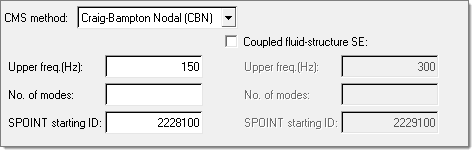
In the CMS Modal Frequency step, define the CMS modal frequency.
For CMS method, select a type of CMS SE.
Choose Craig-Bamption (CBN) to create a
fixed boundary Craig-Bamption (CBN) CMS superelement.
Choose GM - general modal method to
create a mixed (free-free or fixed) boundary (GM - general modal
method) CMS superelement.
Define the modes to be included by specifying either the upper
frequency or the number of modes, as well as Spoint starting IDs to be
assigned to the modes.
The Spoint ID fields are auto filled with the first available ID
provided by the HyperMesh database. Each
mode added to the CMS SE will be assigned a Spoint ID sequentially from
the starting ID, and the total number of Spoint IDs actually used will
be the same as the number of modes found.
Fluid modes, as well as fluid-structure coupling matrix can be included
in the CMS SE by selecting the Coupled fluid-structure
SE checkbox, and providing the above mentioned frequency
and Spoint ID definition for the fluid modes.
Once the task has been completed, click Apply to proceed.
Figure 9.
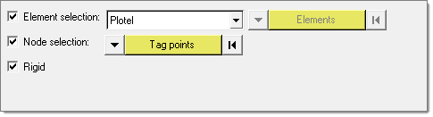
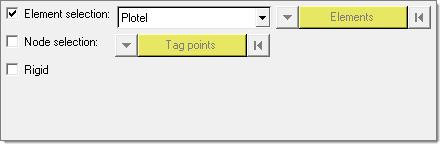
In the CMS Modal Definition task, specify what recovery information is to be
stored in the CMS SE.
Select a set of elements, for which the keyword Plotel is a valid
specification, or a set of grids.
To exclude/include rigid elements from the recovery set, select the
Rigid checkbox.
Once the model recovery set has been defined, click Apply to proceed.
Figure 10.
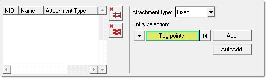
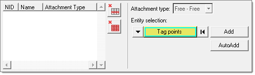
In the Attachment Definition task, specify attachment point sets.
Both fixed and free-free attachments can be specified for a mixed (GM)
CMS SE, while only fixed attachments can be specified for a fixed (CBN)
CMS SE.
Once the attachment set has been defined, click Apply to proceed.
Figure 11.
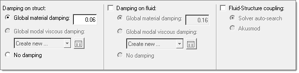
In the MISC Options task, specify structural damping and fluid-structure
coupling options.
You can specify a global material damping to be assigned to all
structural parts, or select the option of No
damping to avoid adding any damping globally if damping
has been specified at the material level for all components.
Note:
Global modal viscous damping or global fluid damping cannot be
stored in a CMS SE, but can be applied in assembly (residual)
runs using the CMS SE as a component.
For fluid-structure coupling, choose Solver
auto-search driven by the ACMODL card, or
Akusmod which assumes that coupling is
provided in a binary file named ftn.70.
Figure 12.
In the Parameter Selection task, select typical solution parameters, such as
title, singular point constraints, and so on.
Check all boxes under the Active column to activate the desired
solution option.
Once the parameters have been selected, click Apply and an Process Manager message box pops up informing you
that the process has come to an end.
Click Yes to close the template, or
No to review or edit the process steps.
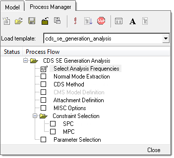
Setup CDS SE Generation Process
Generate a CDS SuperElement (SE) from a finite element based model.
Figure 13.
From the menu bar, click Tools > Freq Resp Process > CDS SE Generation.
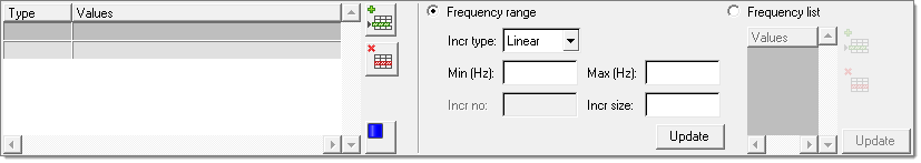
In the Select Analysis Frequencies task, enter the frequencies for which
response solution is needed.
Define the frequency set.
To define the min, max, and a linear step, select
Frequency range. For Incr type,
select Linear and then fill in the
required fields.
To define min, max, and a number of increments with
logarithmic spacing, select Frequency
range. For Incr type, select
Logarithmic and then fill in the
required fields.
To define an arbitrary list of frequencies, select
Frequency list and enter a list
of arbitrary frequencies.
Click Update.
A frequency set entry is created in the list box to the left. You can
add additional frequency sets, or delete one from the list using the
Add row and Delete row icons to the right of the list.
Once the frequency set(s) have been defined, click Apply to proceed.
Figure 14.
In the Normal Mode Extraction task, the default frequencies filled in are based
on the max. frequency you filled in for the previous step.
Modify the values based on the specific requirements of the case under
study.
These values are merely the suggested values based on general use
cases.
Click Apply to
proceed.
Figure 15.
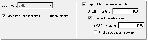
In the CDS Method task, define the CDS method.
For CDS method, select a type of CDS SE.
Currently only the BME method is available.
To store transfer functions in CDS superelement, select the
Store transfer functions in CDS superelement
checkbox.
To generate a CMS-SE modal model result file after solving, select the
Export CMS superelement file checkbox.
Click Apply to
proceed.
Figure 16.
In the CMS Model Definition task, specify which
recovery information is to be stored in the CMS SE.
Restriction: This task is only activated when the Export
CMS superelement file checkbox is selected.
Select a set of elements, for which Plotel is a valid specification, or
a set of grids.
To include or exclude rigid elements from the recovery set, select the
Rigid checkbox.
Once the model recovery set has been defined, click Apply to proceed.
Figure 17.
In the Attachment Definition task, specify attachment point sets.
Both fixed and free-free attachments can be specified for a mixed (GM)
CMS SE, while only fixed attachments can be specified for a fixed (CBN)
CMS SE.
Once the attachment set has been defined, click Apply to proceed.
Figure 18.
In the MISC Options task, specify structural damping and fluid-structure
coupling options.
You can specify a global material damping to be assigned to all
structural parts, or select the option of No
damping to avoid adding any damping globally if damping
has been specified at the material level for all components.
Note:
Global modal viscous damping or global fluid damping cannot be
stored in a CMS SE, but can be applied in assembly (residual)
runs using the CMS SE as a component.
For fluid-structure coupling, choose Solver
auto-search driven by the ACMODL card, or
Akusmod which assumes that coupling is
provided in a binary file named ftn.70.
Figure 19.
In the Parameter Selection task, select typical solution parameters, such as
title, singular point constraints, and so on.
Check all boxes under the Active column to activate the desired
solution option.
Once the parameters have been selected, click Apply and an Process Manager message box pops up informing you
that the process has come to an end.
Click Yes to close the template, or
No to review or edit the process steps.
Figure 20.
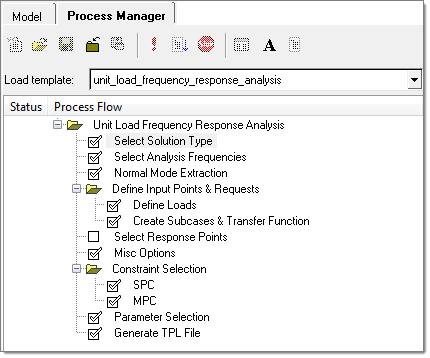
Setup Unit Input Frequency Response Process
Set up subcases with unit inputs. In practice, this is common to generate vibration
and noise sensitivity results.
Figure 21.
From the menu bar, click Tools > Freq Resp Process > Unit Input Frequency Response.
In the Select Solution Type task, select a solution method.
Select either the Direct Frequency Response
solution method, or the Modal Frequency
Response solution method. For large problems involving
more than a few frequencies, the modal solution is typically the most
efficient solution.
Click Apply to
proceed.
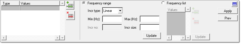
In the Select Analysis Frequencies task, enter the frequencies for which
response solution is needed.
Define the frequency set.
To define the min, max, and a linear step, select
Frequency range. For Incr type,
select Linear and then fill in the
required fields.
To define min, max, and a number of increments with
logarithmic spacing, select Frequency
range. For Incr type, select
Logarithmic and then fill in the
required fields.
To define an arbitrary list of frequencies, select
Frequency list and enter a list
of arbitrary frequencies.
Click Update.
A frequency set entry is created in the list box to the left. You can
add additional frequency sets, or delete one from the list using the
Add row and Delete row icons to the right of the list.
Once the frequency set(s) have been defined, click Apply to proceed.
Figure 22.
In the Normal Mode Extraction task, the default frequencies filled in are based
on the max. frequency you filled in for the previous step.
Modify the values based on the specific requirements of the case under
study.
These values are merely the suggested values based on general use
cases.
Click Apply to
proceed.
Figure 23.
In the Define Input Points & Requests, Define Loads task, define what type
of load is applied.
The first four types are only applicable for structural nodes, and the last
one for fluid nodes.
For Load type, select Force, Enforced
motion (displacement, velocity, or acceleration), or
Acoustic source.
Use the Nodes selector to select nodes, a node set, or tags in the
modeling window, then click
Add.
The table on the left hand side is populated with additional
degree of freedom (DOF) checkboxes.
You can make a single or multiple row selection within the table, and
then right-click to access the DOF row selection options. Alternatively,
make a single or multiple row selection within the table, and then
right-click to access the column selection options.
All selected DOFs will be checked to indicate locations and
directions where unit input are to be applied.
Click Apply to
proceed.
One loadcase will be created for each DOF
indicated.
Figure 24.
In the Define Input Points & Requests, Create Subcases & Transfer
Function task, select to output transfer function between input points.
Of particular interest are driving point (response taken at the same point as
input) transfer functions, which are commonly used as a measure for local
dynamic stiffness, or full matrix (all possible pairs of input point
combinations) output, which is sometimes used as input for FRF based
substructuring analysis.
It is also possible to create new subcase groups of input to be used in
individual subcases. New subcase groups can be added by clicking the Add
Group icon . You can make
a single or multiple row selections within the table, and then select the
newly created Subcase group and click Update. All
input dofs belonging to one subcase group will be used as simultaneous
excitations in one subcase. Figure 25.
In the Select Response Points task, select response points for output.
Select a Response type, such as Displacement.
Use the Entity selector to select nodes, a node set, or tags to be
included in a particular response set.
You can add or delete multiple response sets from the list using the
Add row and Delete row
icons to the right of the list. Figure 26.
Under Output data format, select the complex frequency response data
format (real/imaginary or magnitude/phase).
Under Output file format, select the output file format (h3d, punch, or
op2).
Once all the required responses have been defined, click
Apply to
proceed.
Figure 27.
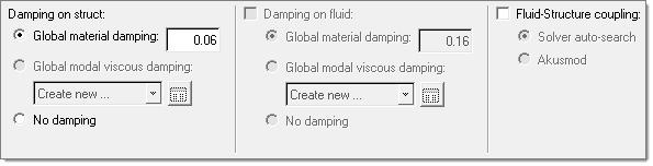
In the Misc Options task, select from the damping options that are available,
including the global modal viscous damping on the structure side, and global
material and viscous damping on the fluid side.
Figure 28.
In the Constraint selection, SPC task, select the boundary condition of the
frequency response analysis.
You can select existing SPCs by checking the corresponding box under
the Active column, or click Create SPC to go to
the Constraints panel and define a new SPC.
Once the boundary condition has been fully defined, click
Apply to
proceed.
Figure 29.
In the Constraint selection, MPC task, select MPC equations to turn on for the
frequency response analysis.
Select existing MPCs by checking the corresponding box under the Active
column.
Once the MPC equations have been selected, click Apply to proceed.
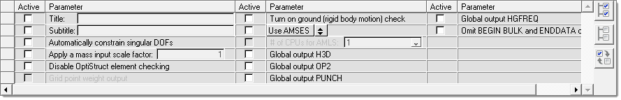
In the Parameter Selection task, select typical solution parameters, such as
title, singular point constraints, and so on.
Check all boxes under the Active column to activate the desired
solution option.
Once the parameters have been selected, click Apply and an Process Manager message box pops up informing you
that the process has come to an end.
Click Yes to close the template, or
No to review or edit the process steps.
Figure 30.
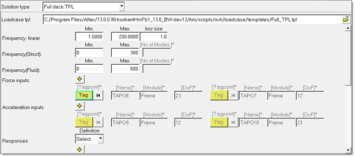
In the Generate TPL file task, generate and save the parameters defined in a
standard template file at your selected location.
Choose Full deck TPL to access the file that has
all of the parameters for the complete unit load FRF process manager. In the
Analysis Manager, the generated template file can be selected as loadcase
for the Solution type Full deck TPL and solver decks can be exported for the
unit FRF. Figure 31.
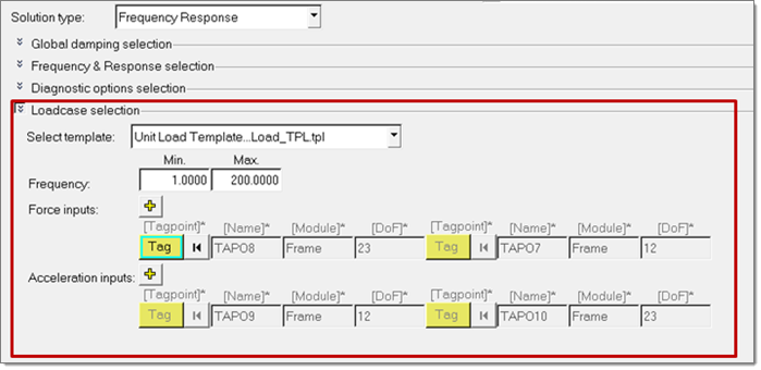
Choose Loads Only TPL to access the file that
contains only the parameters for the loadcase portion of the unit load FRF
process manager. In the Analysis Manager, the generated template file can be
selected as the loadcase for the Solution type Frequency Response and solver
decks can be exported for general FRF. Figure 32.
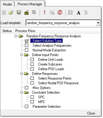
Setup Random PDS Frequency Response Process
Perform random frequency response analysis.
This analysis includes two steps, the first step is to define unit input frequency
response subcase, and the second is to perform random response analysis by combining
the unit input subcases with the auto and cross PSD matrix. Figure 33.
From the menu bar, click Tools > Freq Resp Process > Random PSD Frequency Response.
In the Select Solution Type task, select a solution method.
Select either the Direct Frequency Response
solution method, or the Modal Frequency
Response solution method. For large problems involving
more than a few frequencies, the modal solution is typically the most
efficient solution.
Click Apply to
proceed.
In the Select Analysis Frequencies task, enter the frequencies for which
response solution is needed.
Define the frequency set.
To define the min, max, and a linear step, select
Frequency range. For Incr type,
select Linear and then fill in the
required fields.
To define min, max, and a number of increments with
logarithmic spacing, select Frequency
range. For Incr type, select
Logarithmic and then fill in the
required fields.
To define an arbitrary list of frequencies, select
Frequency list and enter a list
of arbitrary frequencies.
Click Update.
A frequency set entry is created in the list box to the left. You can
add additional frequency sets, or delete one from the list using the
Add row and Delete row icons to the right of the list.
Once the frequency set(s) have been defined, click Apply to proceed.
Figure 34.
In the Normal Mode Extraction task, the default frequencies filled in are based
on the max. frequency you filled in for the previous step.
Modify the values based on the specific requirements of the case under
study.
These values are merely the suggested values based on general use
cases.
Click Apply to
proceed.
Figure 35.
In the Define Input Points, Define Unit Loads task, define what type of load is
applied.
The first four types are only applicable for structural nodes, and the last
one for fluid nodes.
For Load type, select Force, Enforced
motion (displacement, velocity, or acceleration), or
Acoustic source.
Use the Nodes selector to select nodes, a node set, or tags in the
graphics window, then click Add.
The table on the left hand side is populated with additional
degree of freedom (DOF) checkboxes.
You can make a single or multiple row selection within the table, and
then right-click to access the DOF row selection options. Alternatively,
make a single or multiple row selection within the table, and then
right-click to access the column selection options.
All selected DOFs will be checked to indicate locations and
directions where unit input are to be applied.
Click Apply to
proceed.
One loadcase will be created for each DOF
indicated.
Figure 36.
In the Define Input Points, Create Subcases task, select to output transfer
function between input points.
Of particular interest are driving point (response taken at the same point as
input) transfer functions, which are commonly used as a measure for local
dynamic stiffness, or full matrix (all possible pairs of input point
combinations) output, which is sometimes used as input for FRF based
substructuring analysis.
It is also possible to create new subcase groups of input to be used in
individual subcases. New subcase groups can be added by clicking the Add
Group icon . You can make
a single or multiple row selections within the table, and then select the
newly created Subcase group and click Update. All
input dofs belonging to one subcase group will be used as simultaneous
excitations in one subcase. Figure 37.
In the Define Input Points, Define PDS Loads task, input the NxN 2 dimensional
PSD matrix (here N is the number of subcases whose response are used in the
random PSD calculations.
The diagonal cells are used to define auto PSD terms, and the off
diagonal cells are used to define cross PSD terms. For cross PSD, only
the bottom triangle of the matrix needs to be defined. To input a PSD
term, click one of the cells, and then specify the real and imaginary
scaling factor and the frequency table.
Once the PSD matrix input is completed, click Apply to proceed.
Figure 38.
In the Define Responses, Select Response Points task, select response points
for output.
Select a Response type, such as Displacement.
Use the Entity selector to select nodes, a node set, or tags to be
included in a particular response set.
You can add or delete multiple response sets from the list using the
Add row and Delete row
icons to the right of the list. Figure 39.
Under Output data format, select the complex frequency response data
format (real/imaginary or magnitude/phase).
Under Output file format, select the output file format (h3d, punch, or
op2).
Once all the required responses have been defined, click
Apply to
proceed.
Figure 40.
In the Define Responses, Select Nodal PSD Response task, define the response
points and DOFs to be output.
Response points and DOFs can be output into the following formatted files:
XYPUNCH, XYPLOT, and XYPEAK.
Select a response type and then select nodes, set of nodes, or tags,
and then click Add.
The list box is populated to allow you to further the selection
to a set of DOFs. Figure 41.
For each DOF, select the output formats.
Figure 42.
Once the PSD response selection is completed, click Apply to proceed.
In the Misc Options task, select from the damping options that are available,
including the global modal viscous damping on the structure side, and global
material and viscous damping on the fluid side.
Figure 43.
In the Constraint selection, SPC task, select the boundary condition of the
frequency response analysis.
You can select existing SPCs by checking the corresponding box under
the Active column, or click Create SPC to go to
the Constraints panel and define a new SPC.
Once the boundary condition has been fully defined, click
Apply to
proceed.
Figure 44.
In the Constraint selection, MPC task, select MPC equations to turn on for the
frequency response analysis.
Select existing MPCs by checking the corresponding box under the Active
column.
Once the MPC equations have been selected, click Apply to proceed.
In the Parameter Selection task, select typical solution parameters, such as
title, singular point constraints, and so on.
Check all boxes under the Active column to activate the desired
solution option.
Once the parameters have been selected, click Apply and an Process Manager message box pops up informing you
that the process has come to an end.
Click Yes to close the template, or
No to review or edit the process steps.
Figure 45.
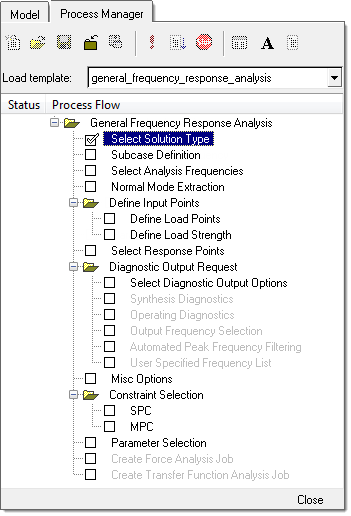
Setup General Frequency Response Process
Apply loads at multiple DOFs simultaneously with arbitrary magnitude and delay
(relative phase).
In the Unit Input Frequency Response process and the Random PSD Frequency Response
processes, loads are limited to single DOF with unit inputs subcases. Figure 46.
From the menu bar, click Tools > Freq Resp Process > General Frequency Response.
In the Select Solution Type task, select a solution method.
Select either the Direct Frequency Response
solution method, or the Modal Frequency
Response solution method. For large problems involving
more than a few frequencies, the modal solution is typically the most
efficient solution.
Click Apply to
proceed.
In the Subcase Definition task, create a new subcase or edit an existing
subcase.
Create or edit a subcase.
To create a new subcase, edit the optional subcase label and
click Add.
To edit an existing subcase, highlight an existing subcase in
the list box, edit the optional subcase label and click
Update.
Once input to the task is complete, click Apply to proceed.
Figure 47.
In the Select Analysis Frequencies task, enter the frequencies for which
response solution is needed.
Define the frequency set.
To define the min, max, and a linear step, select
Frequency range. For Incr type,
select Linear and then fill in the
required fields.
To define min, max, and a number of increments with
logarithmic spacing, select Frequency
range. For Incr type, select
Logarithmic and then fill in the
required fields.
To define an arbitrary list of frequencies, select
Frequency list and enter a list
of arbitrary frequencies.
Click Update.
A frequency set entry is created in the list box to the left. You can
add additional frequency sets, or delete one from the list using the
Add row and Delete row icons to the right of the list.
Once the frequency set(s) have been defined, click Apply to proceed.
Figure 48.
In the Normal Mode Extraction task, the default frequencies filled in are based
on the max. frequency you filled in for the previous step.
Modify the values based on the specific requirements of the case under
study.
These values are merely the suggested values based on general use
cases.
Click Apply to
proceed.
Figure 49.
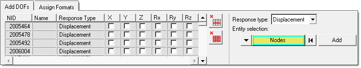
In the Define Input Points, Define Load Points task, define what type of load
is applied.
The first four types are only applicable for structural nodes, and the last
one for fluid nodes.
For Load type, select Force, Enforced
motion (displacement, velocity, or acceleration), or
Acoustic source.
Use the Nodes selector to select nodes, a node set, or tags in the
modeling window, then click
Add.
The table on the left hand side is populated with additional
degree of freedom (DOF) checkboxes.
You can make a single or multiple row selection within the table, and
then right-click to access the DOF row selection options. Alternatively,
make a single or multiple row selection within the table, and then
right-click to access the column selection options.
All selected DOFs will be checked to indicate locations and
directions where unit input are to be applied.
Click Apply to
proceed.
One loadcase will be created for each DOF
indicated.
Figure 50.
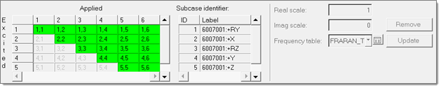
In the Define Input Points, Define Load Strength task, define frequency
dependent load strength and delay for individual subcases or DOFs in one
subcase.
For subcase based definition, once the subcase is selected, select a DOF
row from the list box, and then add load strength frequency tables in either
real/imaginary or magnitude/phase form.
Delay or phase relative to a
reference input DOF can optionally be specified as well. Loading
strength can be defined manually, with external files in csv/text format
and also universal (.unv) files from external data
acquisition tools like LMS, IDEAS, and B&K. Import the
.csv/text or universal file, select the
relevant loading strength and click Save to
define it. You can select one of the radio buttons on the right to
control how the definitions provided are filled into various rows. It is
also possible to go back to the Subcase Definition panel by clicking the
Create Subcase icon to add new subcases or edit existing subcases. If subcases are added
or edited, then you will be redirected to the Select Analysis
Frequencies task to repeat all the steps prior to defining load
strengths. If subcases are not edited then you will come back to the
Define Load Strength task. Figure 51.
For DOF based definition, once the DOF is selected, select a subcase row
from the list and follow the same process described in the above section.
With this option it is not possible to add or edit subcases. Figure 52.
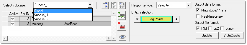
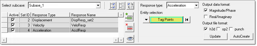
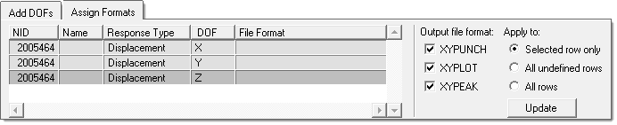
In the Select Response Points task, select response points for output.
Response selection can be global or subcase specific.
Select a Response type, such as Displacement.
Figure 53.
Use the Entity selector to select nodes, a node set, or tags to be
included in a particular response set.
You can add or delete multiple response sets from the list using the
Add row and Delete row
icons to the right of the list. Figure 54.
Under Output data format, select the complex frequency response data
format (real/imaginary or magnitude/phase).
Under Output file format, select the output file format (h3d, punch, or
op2).
Once all the required responses have been defined, click
Apply to
proceed.
Responses selected for the global subcase are by default available for other
individual subcases. Additional responses can be added and used for an
individual subcase. It is also possible to add duplicate response types to
any individual subcase, in addition to those in the global subcase. In this
case a separate response set will be created for that subcase which will be
a union of entities in global and individual subcases. Figure 55.
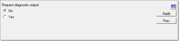
In the Diagnostic Output Request, Select Diagnostic Output Options task,
control if diagnostic outputs are to be generated.
Select No to generate diagnostic output requests
and the process will go directly to the Miscellaneous Options task.
Select Yes to request diagnostic output only at
selected response peaks.
Click Apply to
proceed.
Figure 56.
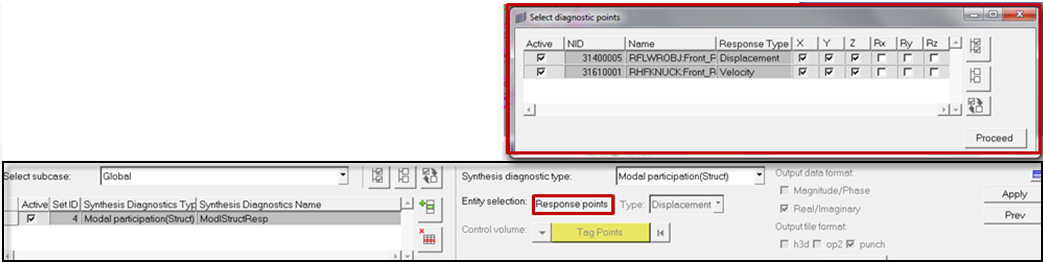
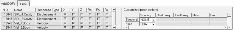
In the Select Diagnostic Output Request, Synthesis Diagnostics task, select the
Synthesis diagnostic type which presents a breakdown (participation factors) to
the response, such as modal participations.
This type will be output only at the peak frequencies of the corresponding
response DOF. The selection of the Synthesis diagnostic type can be Global or
Subcase Specific.
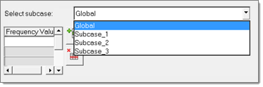
First select the subcase, either Global or
Individual Subcase.
Select response DOFs by clicking Response
points.
In a case of individual subcases the list of responses will be a union
of response entities for Global and Individual Subcase. There is a
specific option of Attachment points on control
volume in Auto TPA and Traditional TPA. In Auto TPA you
can select a connection node set. The elements attached to connection
nodes are automatically segregated into Non-Rigid Element set (CONEL)
and Rigid Element set (CONREL) based on the element type. In Traditional
TPA, you can create a node set at which attachment forces are to be
calculated in the assembled state. Figure 57.
Selecting Traditional TPA as the diagnostic type enables Create
Force Analysis Job and Create Transfer Function Analysis Job tasks in
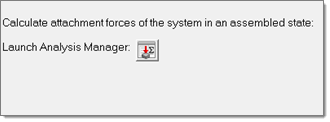
the process manager tree. Create Force Analysis Job allows you to export
a solver deck or submit the job related to the first step of traditional
TPA for calculating attachment forces in the fully assembled state
through the Analysis Manager. Figure 58.
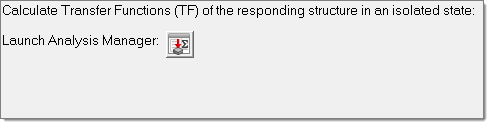
Click Apply to invoke
the Create Transfer Function Analysis Job task.
This will delete all the created entities, and entities related to
unit transfer functions are created. This allows you to export the
solver deck or submit a job related to the second step of TPA for
calculating transfer function in Control Volume through the Analysis
Manager. Figure 59.
In the Select Diagnostic Output Request, Operating Diagnostics task, select the
Operating diagnostic type which is not response specific, such as ODS animation
or energy.
Output in this case will be generated at the super set of the peak frequencies
of all selected response DOFs. In this case the selection of operating
diagnostic type can be global or subcase specific. Figure 60.
In the Select Diagnostic Output Request, Output Frequency Selection task,
control to select frequency at which diagnostic output is to be requested.
Select Automated Peak Frequency Filtering to
customize options used to define response peak frequencies through the
PEAKOUT card.
Select User Specified Frequency List to enter a
list of frequencies for each subcase, which will be referenced by a OFREQ
card in a separate diagnostic output subcase.
In the Select Diagnostic Output Request, Automated Peak Frequency Filtering
task, select the customized options specific for structural and acoustic
responses to be used for selected response peak frequencies.
Select customized options.
Frequency selection for this option can also be global or subcase
specific. The PEAKOUT card specified for the Global subcase is also used
for those subcases for which a separate PEAKOUT card is not specified.
For those subcases where specific peak frequency selection control is
needed, a separate PEAKOUT card should be specified with appropriate
parameters. Figure 61.
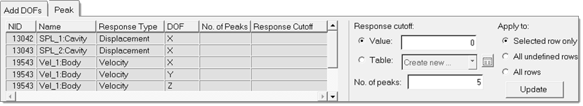
Specify a single threshold value or a frequency table.
Only peaks above the threshold are retained in the search process as
candidates.
Specify the number of peaks (default =5) per response DOF to be kept in
the peak frequency set.
Figure 62.
In the Select Diagnostic Output Request, User Specified Frequency List task,
specify a list of frequencies at which diagnostic output is requested.
This definition is subcase specific. For subcases where a Frequency List is
entered in the Select Analysis Frequencies task, the same frequency list
values are automatically entered by default. Figure 63.
In the Misc Options task, select from the damping options that are available,
including the global modal viscous damping on the structure side, and global
material and viscous damping on the fluid side.
Figure 64.
In the Constraint selection, SPC task, select the boundary condition of the
frequency response analysis.
You can select existing SPCs by checking the corresponding box under
the Active column, or click Create SPC to go to
the Constraints panel and define a new SPC.
Once the boundary condition has been fully defined, click Apply
to proceed.
Figure 65.
In the Constraint selection, MPC task, select MPC equations to turn on for the
frequency response analysis.
Select existing MPCs by checking the corresponding box under the Active
column.
Once the MPC equations have been selected, click Apply to proceed.
In the Parameter Selection task, select typical solution parameters, such as
title, singular point constraints, and so on.
Check all boxes under the Active column to activate the desired
solution option.
Once the parameters have been selected, click Apply and an Process Manager message box pops up informing you
that the process has come to an end.
Click Yes to close the template, or
No to review or edit the process steps.
 . You can make
a single or multiple row selections within the table, and then select the
newly created Subcase group and click Update. All
input dofs belonging to one subcase group will be used as simultaneous
excitations in one subcase.
. You can make
a single or multiple row selections within the table, and then select the
newly created Subcase group and click Update. All
input dofs belonging to one subcase group will be used as simultaneous
excitations in one subcase.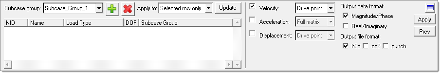
 to add new subcases or edit existing subcases. If subcases are added
or edited, then you will be redirected to the Select Analysis
Frequencies task to repeat all the steps prior to defining load
strengths. If subcases are not edited then you will come back to the
Define Load Strength task.
to add new subcases or edit existing subcases. If subcases are added
or edited, then you will be redirected to the Select Analysis
Frequencies task to repeat all the steps prior to defining load
strengths. If subcases are not edited then you will come back to the
Define Load Strength task.