Adhesion Model and Single Phase Surface Tension Models

Both single phase surface tension and adhesion modeling is based on the work of Akinci et al.

Tartakovsky Model

The Tartakovsky model is based on [8]. In principle it uses the same approach as the Akinci model (see below), which is an inter-particle force that mimics the surface tension effect. The difference with respect to the Akinci model is that the Tartakovsky model derives an expression which is scaling the inter-particle force in such a way that physical (or close to physical) values of the surface tension coefficient could be used. This is meant to avoid the tuning of the numerical parameters, as is the case in the Akinci model.

It is important to note that for the Tartakovsky model to work correctly, appropriate speed of sound (compressibility of the fluid) should be selected. Furthermore, exact implementation from the paper requires an interaction radius of 6*dx (6 particles in size). For performance and infrastructural reasons, in nanoFluidX the radius is limited to 3*dx (3 particles in size). This may have a limited impact on the fidelity of the results in certain situations.

For further reading refer to [8].

Akinci Models

Both Single phase surface tension and adhesion modeling is based on the work of Akinci et. al. [3]. Both models are capable of reproducing qualitatively realistic results, but are in principle unphysical and cannot be generalized for an arbitrary case/simulation. Because of this, trial-and-error tuning of the surface tension coefficient and the adhesion coefficient is necessary if realistic fluid behavior is to be achieved.

Both adhesion and single phase surface tension models rely on a form inter-particle force, which binds the particles together. The way the force is modeled is through a specific kernel shape which mimics a potential energy well. In that sense, particles tend to keep a certain distance from each other and introduce elastic forcing if the particles get too close or too far from each other.

The equation that dictates the adhesion force is given by:(1)

F_{a d} = - \sum_{n b r s} β m_{i} W_{A k} V_{i} \frac{Δ x_{i j}}{| Δ x_{i j} |}

While the single phase surface tension is defined by:(2)

F_{c o h} = - \sum_{n b r s} \frac{2 ρ_{0}}{ρ_{i} + ρ_{j}} γ m_{i}^{2} W_{C o h} \frac{Δ x_{i j}}{| Δ x_{i j} |}

Where,

Indicies $A d$ and $C o h$: Stand for adhesion and cohesion.
$W$: Is the appropriate kernel used for each of the forces.
$m$: Is the mass of the particle.
$Δ x_{i j}$: Is the distance between two interacting particles.
$ρ_{i}$ and $ρ_{j}$: Are instantaneous particle densities.
$ρ_{o}$: Is the default density value of the particle phase.
$β$: Is the adhesion coefficient.
$γ$: Is the cohesion or surface tension coefficient.

The

β

parameter is specified for each WALL or MOVINGWALL phase. That means that the level of adhesion can be different for every WALL or MOVINGWALL phase. The same applies to the

γ

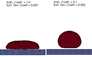
value for the surface tension forces. The balance between surface tension and adhesion forces can replicate qualitatively the physical contact angles between the fluid and the solid elements. An example of balancing adhesion and surface tension forces is shown in Figure 1.

The adhesion model can be used in conjunction with the more physical multiphase surface tension model. In that situation, the surface tension forces are physical and only the adhesion model is left to be tuned, which can be a significantly easier exercise.

Modeling physical behaviour of single phase surface tension and adhesion

In order to partially ease the burden on the user, nanoFluidX team has performed a number of tests resulting in the development of consistent single phase surface tension and adhesion behaviour. By consistency it is meant that if appropriate/desired behaviour is found for a given resolution and a given surface tension or adhesion coefficient – such behaviour can be replicated for other resolutions by following the below methodology.

The simulation data show that the variations of surface tension coefficient $σ$ and adhesion coefficient $ϵ$ due to particle spacing $d x$ changes can be modeled as $α d x^{- β}$ . $α$ and $β$ are case dependent and will take different values depending on the resolution and specific phenomena of the simulation. It is recommended to set $β = 0.7$ and $0.95$ for surface tension and adhesion, respectively.

The procedure to obtain new

σ

or when

d x

changes is as follows:

Assume your current values are $d x_{c}$ , $σ_{c}$ , and $ϵ_{c}$ .
You have a new $d x_{n}$ and wish to find $σ_{n}$ and $ϵ_{n}$ .
Set $β = 0.7$ for surface tension and use $β = 0.95$ for adhesion.
Use $d x_{c}$ and $σ_{c}$ or $ϵ_{c}$ and solve for $α$ .
For example:(3)
$α = \frac{σ_{c}}{d x_{c}^{0.7}}$
or (4)
$α = \frac{ϵ_{c}}{d x_{c}^{0.95}}$
Use the $α$ computed above to find $σ_{n}$ or $ϵ_{n}$ .
For example,(5)
$σ_{n} = α d x_{n}^{0.7}$
or (6)
$ϵ_{n} = α d x_{n}^{0.95}$

These approximations are to save time when the user wants to change $d x$ . They are not perfect fits and some iteration maybe needed to find the adequate values.