HS-1090: Define Discrete Size Variables with the Lookup Model

1. Start HyperStudy.
2. Start a new study in the following ways:
   • From the menu bar, click File > New.
   • On the ribbon, click .
3. In the Add Study dialog, enter a study name, select a location for the study, and click OK.
4. Go to the Define Models step.
5. Add a Parameterized File model.
   1. In the work area, click Add Model.
   2. In the Add dialog, select Parameterized File and click OK.
   3. In the Resource column, click .
   4. In the Open File dialog, navigate to your working directory and open the beam.fem file.
   5. In the Altair HyperStudy dialog, click Yes to parameterize the file.
      The Editor opens.
   6. In the Find area, enter PSHELL and click until you find the PSHELL card.
   7. In the same line as PSHELL, highlight the value 0.002 for the PSHELL thickness.
      Note: In an OptiStruct deck, each field within a card is 8 characters long. Properly select the value for the PSHELL thickness by selecting 0.002 and the three spaces that follow.

      
      
      

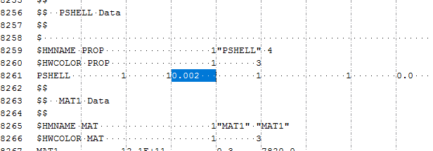
      Figure 1.

   8. Right-click on the highlighted fields and select Create Parameter from the context menu.
   9. In the Parameter: varname_1 dialog, define the parameter and click OK.
      • In the Label field, enter Thickness.
      • For the Upper Bound, enter 0.0022.
      • For the Nominal, enter 0.0020.
      • For the Lower Bound, enter 0.0018.
      • In the Format field, enter %-8.5f.

      
      
      

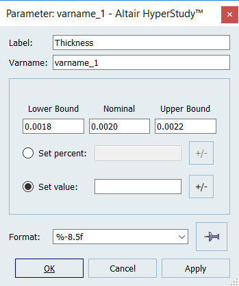
      Figure 2.

   10. Add three more input variables to the template file from the MAT1 card using the information provided in the table below.
       Tip: Quickly highlight 8-character fields by pressing Ctrl to activate the Selector (set to 8 characters) and then clicking the value.

       Parameter	Selection Notification	Selection	Input Variable Label	Lower Bound & Upper Bound	Format
       Young's Modulus	Line number: 8267 Fields: 16 to 24	2.1E+11 & 1 space	Modulus	Lower Bound: 1.9E+011 Upper Bound: 2.3E+011	%-8.1E
       Poisson's Ratio	Line number: 8267 Fields: 32 to 40	0.3 + 5 spaces	Poisson	Lower Bound: 0.27 Upper Bound: 0.33	%-8.2f
       Density	Line number: 8267 Fields: 40 to 48	7820.0 + 2 spaces	Density	Lower Bound: 7038 Upper Bound: 8602	%-8.2f

   11. Click Save.
   12. Click OK to close the Editor.
       The Resource column displays the beam.tpl file, and the Solver input file column displays beam.fem, which is the name of the solver input file HyperStudy writes during any evaluation.
   13. In the Solver execution script column, select OptiStruct (os).

   
   
   

   Figure 3.

6. Add a Lookup model.
   1. In the work area, click Add Model.
   2. In the Add dialog, select Lookup and click OK.
   3. In the Resource column, click .
   4. In the HyperStudy – Load model resource dialog, navigate to your working directory and open the material_prop.csv file.
7. Click Import Variables.
8. In the Import Variables dialog, specify the input variables to import from the material_prop.csv file.
   1. In the Number of design variables field, enter 1.
   2. Click OK.
   The Lookup model automatically populates the input variables based on the number you provided, and you can now identify the material by strings.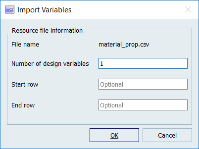

   
   
   

   Figure 4.

9. Go to the Define Input Variables step.
10. Review the four input variables that were imported from the beam.tpl file in the Parameterized File model, and the one input variable that was imported from the material_prop.csv file in the Lookup model.
    Note: The label of fifth input variable has the same label as the first column in the material_prop.csv file, that is Material.

    
    
    

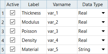
    Figure 5.

1. Go to the Test Models step.
2. Click Run Definition.
   An approaches/setup_1-def/ directory is created inside the study Directory. The approaches/setup_1-def/run__00001/m_1 directory contains the input file, which is the result of the nominal run.

1. Go to the Define Output Responses step.
2. Review the three output responses that were automatically added to the study from the Lookup model, which correspond to the nominal values from the material_prop.csv file.
   Note: The output response labels are the same as the labels in the material_prop.csv file.
3. Click the Data Sources tab.
4. Click Add Data Source to add two data sources.

   
   
   

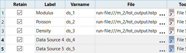
   Figure 6.

5. Define Data Source 4.
   1. In the File field for Data Source 4, click ….
   2. In the Data Source Builder dialog, File field, navigate to the approaches\setup_1-def\run__00001\m_1 directory inside your working directory and open the beam.h3d file.
   3. Set Tool to File Source.
   4. Set Subcase to Subcase 1 (Modal).
   5. Set Type, Request, and Component to Frequency.
   6. Click OK.

   
   
   

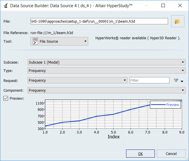
   Figure 7.

6. Define Data Source 5.
   1. In the File field for Data Source 5, click ….
   2. In the Data Source Builder dialog, File field, navigate to the approaches\setup_1-def\run__00001\m_1 directory inside your working directory and open the beam.h3d file.
   3. Set Tool to Read Simulation.
   4. Set Subcase to Subcase 2 (Static).
   5. Set Type to Displacement (Grids).
   6. For Request, set Start to First Request and End to Last Request.
   7. For Components, select MAG.
   8. Set Time to All.
   9. Click OK.
7. Click the Define Output Responses tab.
8. Define the 1st_natural_freq output response.
   1. Click Add Output Response.
   2. In the Label field, enter 1st_natural_freq.
   3. In the Expression field, click ….
   4. In the Expression Builder, click the Data Sources tab.
   5. From the list of data sources, click Data Source 4.
   6. Next to Insert Varname, click and select First Element.

      
      
      

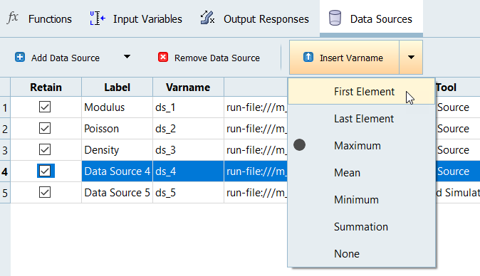
      Figure 8.

   7. Click Insert Varname.
      The Evaluate Expression field displays ds_4[0].
   8. Click OK.
9. Define the Max_disp output response.
   1. Click Add Output Response.
   2. In the Label field, enter Max_disp.
   3. In the Expression field, click ….
   4. In the Expression Builder, click the Data Sources tab.
   5. From the list of data sources, click Data Source 5.
   6. Next to Insert Varname, click and select Maximum.
   7. Click Insert Varname.
      The Evaluate Expression field displays max(ds_5).
   8. Click OK.
10. Click Evaluate to extract the response values.

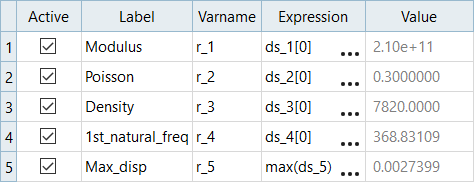
Figure 9.

In this step you will establish links between the input variables imported from the beam.tpl file in the Parameterized File model with the output responses imported from the material_prop.csv file in the Lookup model.

1. Go to the Define Input Variables step.
2. Click the Links tab.
3. Link the Modulus input variable to the Modulus output response.
   1. In the Expression field for Modulus, click ….
   2. In the Expression Builder, click the Output Responses tab.
   3. From the list of output responses, select Modulus.
   4. Click Insert Varname.
   5. Click OK to close the Expression Builder.
4. Create two more links.
   1. Link the Poissons input variable to the Poissons output response.
   2. Link the Density input variable to the Density output response.

   
   
   

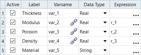
   Figure 10.

5. Go to the Test Models step and click Run Definition.
6. Click the Model Data tab and verify that the input variables are equal to their corresponding linked output response.

   
   
   

   Figure 11.

1. Add a DOE.
   1. In the Explorer, right-click and select Add from the context menu.
   2. In the Add dialog, select DOE and click OK.
2. Go to the DOE 1 > Specifications step.
3. Set the Mode to Modified Extensible Lattice Sequence (Mels) and that the Number of Runs is set to 6.

   
   
   

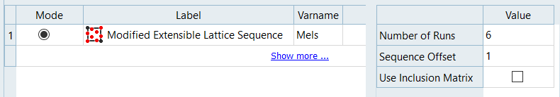
   Figure 12.

4. Click Apply.
5. Go to the DOE 1 > Evaluate step.
6. Click Evaluate Tasks.
7. Go to the DOE 1 > Post-Processing step.
8. Click the Summary tab.

   The output responses (material property numbers) from the .csv file are linked to the input variables (material property set in the FEA deck), and are now controlled in the categorical input variable Material.

   Any number of material data can be added using a library, without requiring you to explicitly create “if” conditions in a .tpl file. This is the advantage of using Lookup model in this case.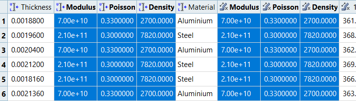

   
   
   

   Figure 13.