HL-T: 1030 Multiaxial Strain-Life (E-N)
In this tutorial you will:
- Import a model to HyperLife
- Select the EN module and define its required parameters
- Create and assign materials
- Assign load histories for scaling the stresses from FEA subcases
- Evaluate and view results
Before you begin, copy the file(s) used in this tutorial to your
working directory.
- HL-1030\Ibeam.h3d
- Load_History_Files\load1.csv
- Load_History_Files\load2.csv
- Load_History_Files\load3.csv
- Load_History_Files\load4.csv
Import the Model
-
From the Home tools, Files tool group, click the Open Model tool.

Figure 1. -
Click Apply.
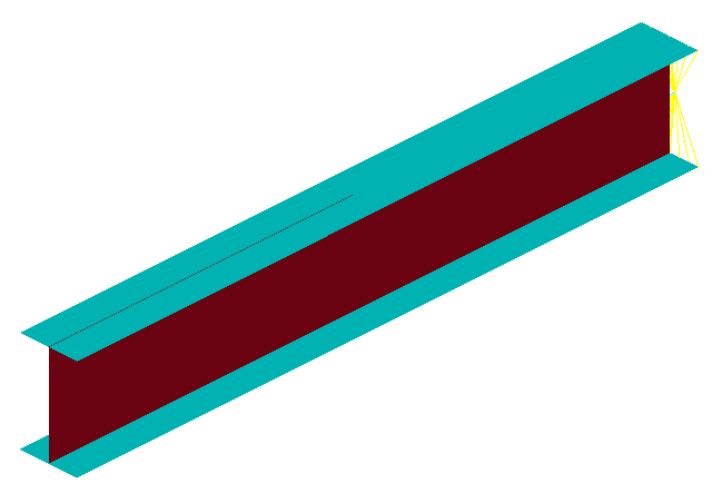
Figure 2.
Tip: Quickly import the model by dragging and
dropping the .h3d file from
a windows browser into the HyperLife
modeling window.
Define the Fatigue Module
-
Click the arrow next to the fatigue module icon and select the
EN tool from the list of options.

Figure 3.The EN dialog opens. -
Define the EN configuration parameters.
- Select Multi Axial as the method.
- Select MPa for the FE model units.
- Enter a value of 20 for the number of planes.
- Enter a value of 0.5 for the certainty of survival.
- Select SWT for the tension damage model.
- Select FS for the shear damage model.
- Select Worst for the layer selection.
- Select Time Series for the type of loading.
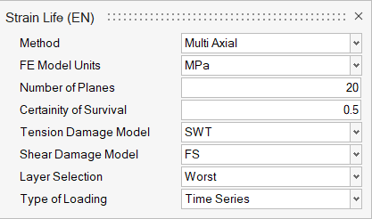
Figure 4.
Assign Materials
-
Click the Material tool.

Figure 5.The Assign Material dialog opens. -
Create a new material.
-
Click
 to create a new material.
-
Accept all other default settings, both in the EN and Other tabs, then
click Plot & Save.
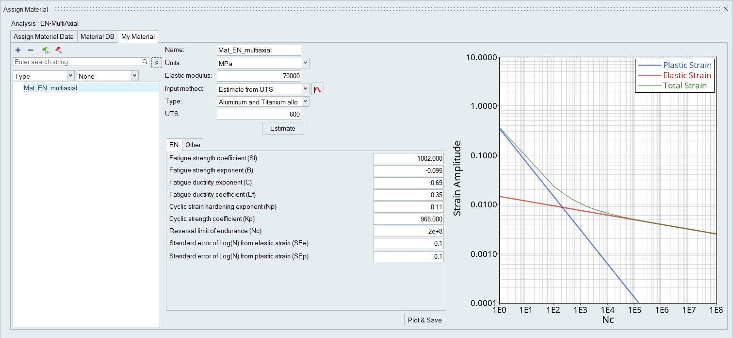
Figure 6.
-
Click
-
Return to the Assign Material Data tab and select
Mat_EN_multiaxial from the Material drop-down menu
for both Flange and Web.
The Material list is populated with the materials selected from Material Database and My Material.
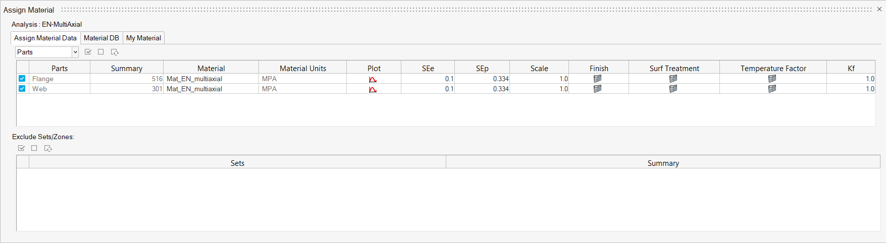
Figure 7.
Assign Load Histories
-
Click the Load Map tool.

Figure 8.The Load Map dialog opens. -
Click
 in the Choose File
field and browse for load1.csv.
in the Choose File
field and browse for load1.csv.
-
Click to add the load case.
- Optional:
Click
 to view a plot of the loads.
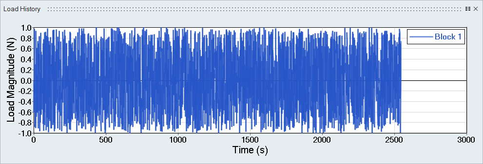
Figure 9. Load 1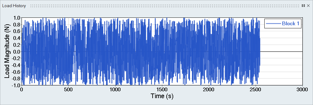
Figure 10. Load 2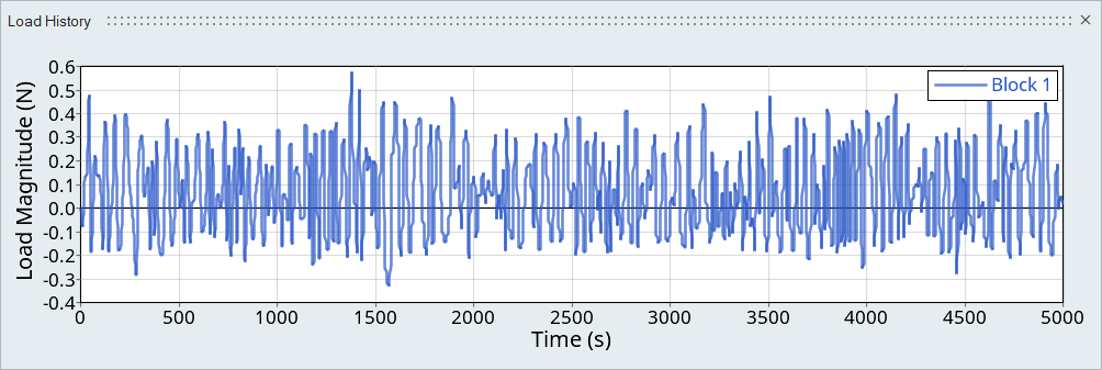
Figure 11. Load 3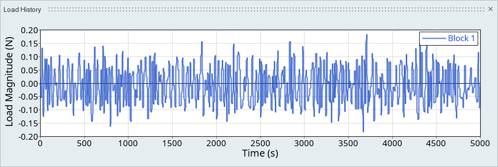
Figure 12. Load 4Tip: Expand the width of the dialog to view a clearer picture of the plot. -
Select both the load 1 (block1) and load 2
(block1) channels and Subcase 1 and
Subcase 2, then click to create the first event.
-
Set the Scale as shown in the image below.
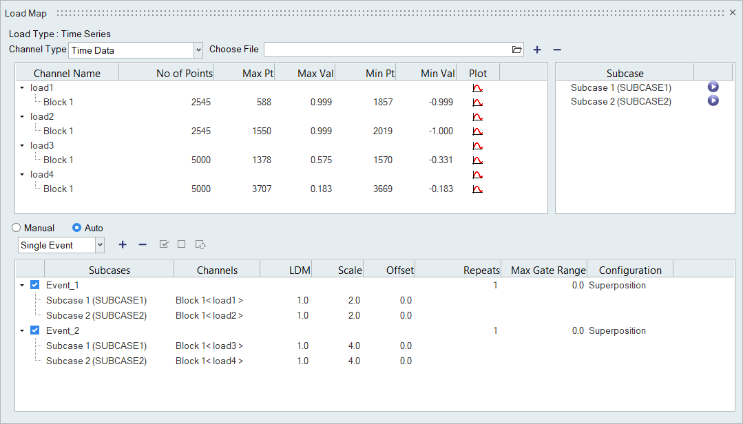
Figure 13.
Evaluate and View Results
-
From the Evaluate tool group, click the
Run Analysis tool.

Figure 14.The Evaluate dialog opens.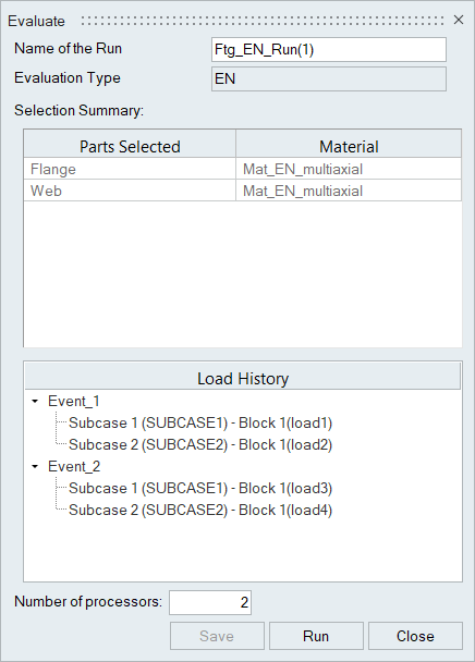
Figure 15. -
Use the Results Explorer to
visualize various types of results.
The contour below highlights the total damage (Event 1 + Event 2).
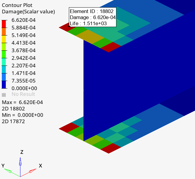
Figure 16.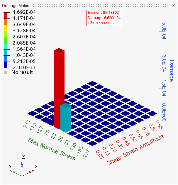
Figure 17. Event 1: Damage matrix for element 18802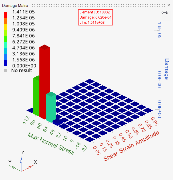
Figure 18. Event 2: Damage matrix for element 18802